This blog post builds on the ideas started in three previous blog posts.
In this blog post I'll show how to deploy the same ML model that we deployed as a batch job in this blog post, as a task queue in this blog post, inside an AWS Lambda in this blog post, as a Kafka streaming application in this blog post, a gRPC service in this blog post, as a MapReduce job in this blog post, as a Websocket service in this blog post, and as a ZeroRPC service in this blog post.
The code in this blog post can be found in this github repo.
Introduction
Data processing pipelines are useful for solving a wide range of problems. For example, an Extract, Transform, and Load (ETL) pipeline is a type of data processing pipeline that is used to extract data from one system and save it to another system. Inside of an ETL, the data may be transformed and aggregated into more useful formats. ETL jobs are useful for making the predictions made by a machine learning model available to users or to other systems. The ETL for such an ML model deployment looks like this: extract features used for prediction from a source system, send the features to the model for prediction, and save the predictions to a destination system. In this blog post we will show how to deploy a machine learning model inside of a data processing pipeline that runs on the Apache Beam framework.
Apache Beam is an open source framework for doing data processing. It is most useful for doing parallel data processing that can easily be split among many computers. The Beam framework is different from other data processing frameworks because it supports batch and stream processing using the same API, which allows developers to write the code one time and deploy it in two different contexts without change. An interesting feature of the Beam programming model is that once we have written the code, we can deploy into an array of different runners like Apache Spark, Apache Flink, Apache MapReduce, and others.
The Google Cloud Platform has a service that can run Beam pipelines. The Dataflow service allows users to run their workloads in the cloud without having to worry about managing servers and manages automated provisioning and management of processing resources for the user. In this blog post, we'll also be deploying the machine learning pipeline to the Dataflow service to demonstrate how it works in the cloud.
Building Beam Jobs
A Beam job is defined as a driver process that uses the Beam SDK to state the data processing steps that the Beam job does. The Beam SDK can be used from Python, Java, or Go processes. The driver process defines a data processing pipeline of components which are executed in the right order to load data, process it, and store the results. The driver program also accepts execution options that can be set to modify the behavior of the pipeline. In our example, we will be loading data from an LDJSON file, sending it to a model to make predictions, and storing the results in an LDJSON file.
The Beam programming model works by defining a PCollection, which is a collection of data records that need to be processed. A PCollection is a data structure that is created at the beginning of the execution of the pipeline, and is received and processed by each step in a Beam pipeline. Each step in the pipeline that modifies the contents of the PCollection is called a PTransform. For this blog post we will create a PTransform component that takes a PCollection, makes predictions with it, and returns a PCollection with the prediction results. We will combine this PTransform with other components to build a data processing pipeline.
Package Structure
The code used in this blog post is hosted in this Github repository. The codebase is structured like this:
-   data ( data for testing job)
-   model_beam_job (python package for apache beam package)
    -   __init__.py
    -   main.py (pipeline definition and launcher)
    -   ml_model_operator.py (prediction step)
-   tests ( unit tests )
-   Makefile
-   README.md
-   requirements.txt
-   setup.py
-   test_requirements.txt
Installing the Model
As in previous blog posts, we'll be deploying a model that is packaged separately from the deployment codebase. This approach allows us to deploy the same model in many different systems and contexts. To install the model package, we'll install the model into the virtual environment. The model package can be installed from a git repository with this command:
pip install git+https://github.com/schmidtbri/ml-model-abc-improvements
Now that we have the model installed in the environment, we can try it out by opening a python interpreter and entering this code:
>>> from iris_model.iris_predict import IrisModel
>>> model = IrisModel()
>>> model.predict({"sepal_length":1.1, "sepal_width": 1.2, "petal_width": 1.3, "petal_length": 1.4})
{'species': 'setosa'}
The IrisModel class implements the prediction logic of the iris_model package. This class is a subtype of the MLModel class, which ensures that a standard interface is followed. The MLModel interface allows us to deploy any model we want into the Beam job, as long as it implements the required interface. More details about this approach to deploying machine learning models can be found in the first three blog posts in this series.
MLModelPredictOperation Class
The first thing we'll do is create a PTransform class for the code that receives records from the Beam framework and makes predictions with the MLModel class. This is the class:
class MLModelPredictOperation(beam.DoFn):
The code above can be found here.
The class we'll be working with is called MLModelPredictOperation and it is a subtype of the DoFn class that is part of the Beam framework. The DoFn class defines a method which will be applied to each record in the PCollection. To initialize the object with the right model, we'll add an __init__ method:
def __init__(self, module_name, class_name):
    beam.DoFn.__init__(self)
    model_module = importlib.import_module(module_name)
    model_class = getattr(model_module, class_name)
    model_object = model_class()
    if issubclass(type(model_object), MLModel) is None:
        raise ValueError("The model object is not a subclass of MLModel.")
    self._model = model_object
The code above can be found here.
We'll start by calling the __init__ method of the DoFn super class, this initializes the super class. We then find and load the python module that contains the MLModel class that contains the prediction code, get a reference to the class, and instantiate the MLModel class into an object. Now that we have an instantiated model object, we check the type of the object to make sure that it is a subtype of MLModel. If it is a subtype, we store a reference to it.
Now that we have an initialized DoFn object with a model object inside of it, we need to actually do the prediction:
def process(self, data, **kwargs):
    yield self._model.predict(data=data)
The code above can be found here.
The prediction is very simple, we take the record and pass it directly to the model, and yield the result of the prediction. To make sure that this code will work inside of a Beam pipeline, we need to make sure that the pipeline feeds a PCollection of dictionaries to the DoFn object. When we create the pipeline, we'll make sure that this is the case.
Creating the Pipeline
Now that we have a class that can make a prediction with the model, we need to build a simple pipeline around it that can load data, send it to the model, and save the resulting predictions.
The creation of the Beam pipeline is done in the run function in the main.py module:
def run(argv=None):
    parser = argparse.ArgumentParser()
    parser.add_argument('--input', dest='input', help='Input file to process.')
    parser.add_argument('--output', dest='output', required=True, help='Output file to write results to.')
    known_args, pipeline_args = parser.parse_known_args(argv)

    pipeline_options = PipelineOptions(pipeline_args)
    pipeline_options.view_as(SetupOptions).save_main_session = True
The code above can be found here.
The pipeline options is an object that is given to the Beam job to modify the way that it runs. The parameters loaded from a command line parser are fed directly to the PipelineOptions object. Two parameters are loaded in the command line parser: the location of the input files, and the location where the output of the job will be stored.
When we are done loading the pipeline options, we can arrange the steps that make up the pipeline:
with beam.Pipeline(options=pipeline_options) as p:
    (p
    | 'read_input' >> ReadFromText(known_args.input, coder=JsonCoder())
    | 'apply_model' >> beam.ParDo(MLModelPredictOperation(module_name="iris_model.iris_predict", class_name="IrisModel"))
    | 'write_output' >> WriteToText(known_args.output, coder=JsonCoder())
    )
The code above can be found here.
The pipeline object is created by providing it with the PipelineOptions object that we created above. The pipeline is made up of three steps: a step that loads data from an LDJSON file and creates a PCollection from it, a step that makes predictions with that PCollection, and a step that saves the resulting predictions as an LDJSON file. The input and output steps use a class called JsonCoder, which takes care of serializing and deserializing the data in the LDJSON files.
Now that we have a configured pipeline, we can run it:
result = p.run()
result.wait_until_finish()
The code above can be found here.
The main.py module is responsible for arranging the steps of the pipeline, receiving parameters, and running the Beam job. This script will be used to run the job locally and in the cloud.
Testing the Job Locally
We can test the job locally by running with the python interpreter:
export PYTHONPATH=./
python -m model_beam_job.main --input data/input.json --output data/output.json
The job takes as input the "input.json" file in the data folder, and produces a file called "output.json" to the same folder.
Deploying to Google Cloud
The next thing we'll do is run the same job that we ran locally in the Google Cloud Dataflow service. The Dataflow service is an offering in the Google Cloud suite of services that can do scalable data processing for batch and streaming jobs. The Dataflow service runs Beam jobs exclusively and manages the job, handling resource management and performance optimization.
To run the model Beam job in the cloud, we'll need to create a project. In the Cloud Console, in the project selector page click on "Create Cloud Project", then create a project for your solution. The newly created project should be the currently selected project, then any resources that we create next will be held in the project. In order to use the GCP Dataflow service, we'll need to have billing enabled for the project. To make sure that billing is working, follow these steps.
To be able to create the Dataflow job, we'll need to have access to the Cloud Dataflow, Compute Engine, Stackdriver Logging, Cloud Storage, Cloud Storage JSON, BigQuery, Cloud Pub/Sub, Cloud Datastore, and Cloud Resource Manager APIs from your new project. To enable access to these APIs, follow this link, then select your new project and click the "Continue" button.
Next, we'll create a service account for our project. In the Cloud Console, go to the Create service account key page. From the Service account list, select "New service account". In the Service account name field, enter a name. From the Role list, select Project -> Owner and click on the "Create" button. A JSON file will be created and downloaded to your computer, copy this file to the root of the project directory. To use the file in the project, open a command shell and set the GOOGLE_APPLICATION_CREDENTIALS environment variable to the full path to the JSON file that you placed in the project root. The command will look like this:
export GOOGLE_APPLICATION_CREDENTIALS=/Users/.../apache-beam-ml-model-deployment/model-beam-job-a7c5c1d9c22c.json
To store the file we will be processing, we need to create a storage bucket in the Google Cloud Storage service. To do this, go to the bucket browser page, click on the "Create Bucket" button, and fill in the details to create a bucket. Now we can upload our test data to a bucket so that it can be processed by the job. To upload the test data click on the "Upload Files" button in the bucket details page and select the input.json file in the data directory of the project.
Next, we need to create a tar.gz file that contains the model package that will be run by the Beam job. This package is special because it cannot be installed from the public Pypi repository, so it must be uploaded along with the Beam job to the Dataflow job. To create the tar.gz file, we created a target in the project Makefile called "build-dependencies". When executed, the target downloads the code for the iris_model package, builds a tar.gz.distribution file, and leaves in the "dependencies" directory.
We're finally ready to send the job to be executed in the Dataflow service. To do this, execute this command:
python -m model_beam_job.main --region us-east1 \
  --input gs://model-beam-job/input.json \
  --output gs://model-beam-job/results/outputs \
  --runner DataflowRunner \
  --machine_type n1-standard-4 \
  --project model-beam-job-294711 \
  --temp_location gs://model-beam-job/tmp/ \
  --extra_package dependencies/iris_model-0.1.0.tar.gz \
  --setup_file ./setup.py
The job is sent by executing the same python scripts that we used to test the job locally, but we've added more command line options. The input and output options work the same as in the local execution of the job, but now they point to locations in the Google Cloud Storage bucket. The runner option tells the Beam framework that we want to use the Dataflow runner. The machine_type option tells the Dataflow service that we want to use that specific machine type when running the job. The project option points to the Google Cloud project we created above. The temp_location option tells the Dataflow service that we want to store temporary files in the same Google Cloud Storage bucket that we are using for the input and output. The extra_package option points to the iris_model distribution tar.gz file that we created above, this file will be sent to the Dataflow service along with the job code. Lastly, the setup_file option points at the setup.py file of the model_beam_job package itself, this allows the command to package up any code files that the job depends on.
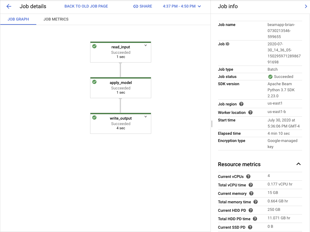
Once we execute the command, the job will be started in the cloud. As the job runs it will output a link to a webpage that can be used to monitor the progress of the job. Once the job completes, the results will be in the Google Cloud Storage bucket that we created above.
Closing
By using the Beam framework, we are able to easily deploy a machine learning prediction job to the cloud. Because of the simple design of the Beam framework, a lot of the complexities of running a job on many computers are abstracted out. Furthermore, we are able to leverage all of the features of the Beam framework for advanced data processing.
One of the important features of this codebase is the fact that it can accept any machine learning model that implements the MLModel interface. By installing another model package and importing the class that inherits from the MLModel base class, we can easily deploy any number of models in the same Beam job without changing the code. However, we do need to change the pipeline definition to change or add models to it. Once again, the MLModel interface allowed us to abstract out the building a machine learning model from the complexity of deploying a machine learning model.
One thing that we can improve about the code is the fact that the job only accepts files encoded as LDJSON. We did this to make the code easy to understand, but we can easily add other options for the format of the input data making the pipeline more flexible and easier to use.