This blog post continues the ideas started in three previous blog posts.
The code in this blog post can be found in this github repo.
Introduction
In previous blog posts I showed how to develop an ML model in such a way that makes it easy to deploy, and I showed how to create a web app that is able to deploy any model that followed the same design pattern. However, not all deployments of ML model are deployed within web apps. In this blog post I deploy the same model used in the previous blog posts as an ETL job.
An ETL job is a procedure for copying data from a source system into a destination system, with some processing along the way. The acronym ETL stands for extract, transform, and load; as in extract from a source system, transform the data into a format compatible with the destination system, and load the resulting data into the destination system. ETLs are most commonly associated with data warehousing systems, in which they are used to take data from a system of record and transform it to make it useful for reporting.
ETL jobs are useful for making predictions available to end users or to other systems. The ETL for such an ML model deployment looks like this: extract features used for prediction from a source system, send the features to the model for prediction, and save the predictions to a destination system.
A big distinction between ML models that are deployed in an ETL job and the Flask web application shown in the previous blog post is that the ETL job is not a real time system since it is not expected to return predictions to the client quickly. ETLs are also meant to process thousands of records at a time, whereas a web app processes one record (request) at a time. A real-time deployment of an ML model should be able to return single predictions in less than a second, an ETL deployment has a looser time constraint but makes many more predictions.
Another distinction between an ETL job deployment and a web service deployment of an ML model is that an ETL saves predictions to data storage, and the predictions are then accessed from there by the users of the predictions. This means that the user of the predictions does not interact with the model directly, and only has access to the predictions saved since the ETL last ran. I call this distinction interactive vs. non-interactive ML models. When an ML model is deployed non-interactively, the users of the predictions have limitations as to how they are able to use the model since they don't have direct access to the model.
Bonobo for ETL Jobs
The bonobo package is a python package for writing ETL jobs, offering a simple pythonic interface for writing code that loads, transforms, and saves data. The package works well for small datasets that can be processed in single processes, but not as useful for larger datasets. Nevertheless, the package is perfect for small scale data processing. The package has a strong object-oriented bend to it and it encourages good software engineering best practices through a well-designed API.
The bonobo package does data processing by running directed acyclic graphs (DAG) of operations defined by the user. I won't get into the complex aspects of what a DAG is in this post, so to define it simply: a DAG of data processing steps is a set of steps that can be executed in a certain order in time based on their dependencies. For example, in order to transform a data record we must first load the record into memory, therefore the Extract step must be done before the Transform step. Each step in a DAG is called a "transformation", a transformation can do one of three things: load data, transform data, or save data.
ETL Application
To develop the ETL application with the Bobobo package I first set up the project structure
- data (folder for test data)
- model_etl (folder for application code)
    - __init__.py
    - etl_job.py
    - model_node.py
- tests (folder for unit tests)
- .gitignore
- Makefile
- README.md
- requirements.txt
- test_requirements.txt
This folder structure can be seen here in the github repository.
This folder structure for the ETL application looks very similar to the one used in the Flask application in the previous blog post. We will be following the same practices as before, adding documentation, unit tests and a Makefile to the application to ensure quality code and to make it easier to use.
MLModelTransformer Class
Running a machine learning model prediction step inside an ETL DAG requires many of the same things as running a model inside a web application. In the previous blog post we managed instances of MLModel classes inside a ModelManager singleton object. The ModelManager object was used by the web application to maintain a list of MLModel objects, and returned information about them on request.
When a model makes a prediction, it is making a transformation on an incoming record and returning a prediction. Therefore, to embed an ML model inside of a bonobo ETL job, we just need to write a transformation. We can write a transformation as a class:
class MLModelTransformer(object):
    def __init__(self, module_name, class_name):
        model_module = importlib.import_module(module_name)
        model_class = getattr(model_module, class_name)
        model_object = model_class()

        if isinstance(model_object, MLModel) is False:
            raise ValueError("The MLModelNode can only hold references to objects of type MLModel.")

        # saving the model reference
        self.model = model_object
The code above can be found here.
The __init__ method receives two parameters: module_name and class_name. The __init__ method uses these parameters to dynamically import and instantiate an MLModel class and saves a reference to the newly created object. The __init__ method also verifies that the class inherits from the MLModel base class.
Just like the ModelManager class from the Flask app, the MLModelTransformation class instantiates and maintains a reference to an MLModel object internally. However, it is not meant to be a singleton object and it only holds one MLModel object.
The MLModelTransformation class is meant to be plugged into a bonobo DAG and exchange data with other transformations in the DAG. For that purpose we implement a __call__ method:
def __call__(self, data):
    try:
        yield self.model.predict(data=data)
    except MLModelSchemaValidationException as e:
        raise e
The code above can be found here.
The __call__() method makes the class a callable. This mechanism is used by the bonobo package to feed data into the DAG transformation and receive data back. The yield keyword allows bonobo to run transformations asynchronously. By implementing the transformer this way, we can compose many different DAGs that use MLModel derived classes to do data transformations.
Now we can test the MLModelTransformation class to make sure it\'s working as expected. First, we have to install a model to the environment, we'll install the iris_model package that was built in a previous blog post:
pip install git+https://github.com/schmidtbri/ml-model-abc-improvements
Now that we have a model package in the environment, we use a Python interactive session to instantiate the class and try to make a prediction:
>>> from model_etl.model_node import MLModelTransformer
>>> model_transformer = MLModelTransformer(module_name="iris_model.iris_predict", class_name="IrisModel")
>>> generator = model_transformer(data={"sepal_length": 4.4,
... "sepal_width": 2.9, "petal_length": 1.4, "petal_width": 0.2})
>>> result = list(generator)
>>> result
[{'species': 'setosa'}]
We first instantiate the transformer class by pointing it at the module and class in the iris_model package that implement the MLModel base class. Then we can make a prediction by calling class with a single dictionary object. The transformers makes predictions by using the yield keyword, so we have to cast the return value of the transformer into a list to view it on the screen.
As in the previous blog posts, we are trying to write the code in such a way as to make it reusable in many situations. The MLModelTransformer class can be used to load and manage ML model objects in any bonobo ETL, which saves time and work later. One caveat to this, however, is that the ETL must feed records to the MLModelTransformer object exactly as the MLModel expects it, since any schema differences will raise a MLModelSchemaValidationException from the model within the transformer. In practice, this means that the IrisModel.predict() method expects to receive data in a dictionary with several floating point numbers, if the data source does not provide records with this schema, we have to transform the incoming data to match it.
Creating a Graph
A bonobo application runs an ETL from a Graph object that is defined at application startup. Any number of transformations can be used, and they can be arranged into complex DAGs. Every Graph object must contain at least one extractor to get data from an outside source, and one loader to save data to an outside destination. The bonobo package provides several options for accessing data files, we'll use the JSONLD extractor and loader transformations to define a simple Graph inside a function:
def get_graph(**options):
    graph = bonobo.Graph()
    graph.add_chain(
        LdjsonReader(options["input_file"], mode='r'),
        MLModelTransformer(module_name="iris_model.iris_predict", class_name="IrisModel"),
        LdjsonWriter(options["output_file"], mode='w'))
    return graph
The code above can be found here.
The function receives two file names as parameters. The input file name is used to instantiate a LDjsonReader object that will load data from a local JSON file, and the output file name is used to instantiate an LdjsonWriter to write data to a local JSON file. The MLModelTransformer class is instantiated by pointing it at the IrisModel class.
We can now instantiate the graph from an interactive Python session:
>>> from model_etl.etl_job import get_graph
>>> graph = get_graph("data/input.json", "data/output.json")
>>> graph
<bonobo.structs.graphs.Graph object at 0x10a52ffd0>
The great thing about this approach to building ETLs is that a different reader or writer can be easily swapped in to add functionality, while the core transformations of the ETL remain unchanged. For example, we can implement a Graph that reads CSV files and writes TSV files in the same module, and select it at runtime using a parameter.
Running the ETL Process Locally
The graph defined in the previous section works well when running it from an interactive Python session, but it would be better to run in from the command line. Before writing the code to create simple command line interface, we need to create some parameters for the input and output file names:
def get_argument_parser(parser=None):
    parser = bonobo.get_argument_parser(parser=parser)
    parser.add_argument("--input_file", "-i", type=str, default=None, help="Path of the input file.")
    parser.add_argument("--output_file", "-o", type=str, default=None, help="Path of the output file.")
    return parser
The code above can be found here.
The function retrieves standard command line parser that is defined by the bonobo package, and adds two parameters for the input and output file names. The new parser object is then returned.
To create a CLI interface we define a __main__ function inside of the etl.py module and use the parser defined above:
if __name__ == '__main__':
    parser = get_argument_parser()
    with bonobo.parse_args(parser) as options:
        bonobo.run(
            get_graph(**options),
            services={}
        )
The code above can be found here.
The graph can now be run from the command line with these commands:
export PYTHONPATH="${PYTHONPATH}:./"
python model_etl/etl_job.py --input_file=data/input.json --output_file=data/output.json
First, we add the current directory to the PYTHONPATH environment variable to ensure that the python modules will be found. Then we can execute the graph with the command line interface in the etl_job.py module and the CLI parameters. The input file is included in the repository here, and contains 15 records, which we can see were processed by the three transformations in the graph. The output will be saved as an LDJSON file in the data folder of the project.
The ETL graph looks pretty good now, it is able to run from the command line and we can parametrize the input and output files. However, a real-world ETL is probably not accessing data from the local hard drive, so we'll add the ability to access data from other places.
Accessing Data from a Service
When testing an ETL job locally, it is easiest to load data from and save data to the local hard drive. When running the ETL in a production environment, the ETL code will most likely be accessing data from remote storage systems. We can easily write an implementation of the LdjsonReader and LdjsonWriter classes to access files from a remote system, but this is not a best practice.
To be able to write code once and reuse it in many different situations, the bonobo package supports dependency injection through service abstractions. A service is a software component that provides functionality to other software components. For example, the os Python package that is part of the standard library can be thought of as a service, since it provides access to the operating system. Dependency injection is a software pattern that allows software components to be written in such a way that makes them easier to reuse in many different situations. For example, a d instance of the os
In the example we set up for this blog post, we are interested in accessing files from a remote data source, but without changing the ETL's Graph. In this way, we can easily change the data source of the ETL in the future without changing the code of the ETL. To show how to do this, I will change the local filesystem as the file source for an S3 bucket, without changing the bonobo Graph object.
The bonobo package provides a mechanism for injecting service instances into a Graph at runtime. Right now, the JSON files are being accessed through a local filesystem service that is injected by default into every Graph. To be able to access files from a remote service, we'll just replace the default filesystem service instance with another service instance with the same interface that loads files from a remote source.
As an example, we'll show how to access files stored in S3. To be able to access files in an S3 bucket, we first have to install the fs-s3fs package with this command:
pip install fs-s3fs
Now we can instantiate a special type of filesystem that accesses files from an AWS bucket but has the same interface as a local filesystem. The fs package already provides this functionality when we accessed the files in the example above, so we know that the code will work with the s3 filesystem.
To inject a service through the bonobo package we define a dictionary like this:
def get_services(**options):
    return {
        'fs': S3FS(options["bucket"],
                   aws_access_key_id=options["key"],
                   aws_secret_access_key=options["secret_key"],
                   endpoint_url=options["endpoint_url"],)
    }
The code above can be found here.
The new fs filesystem service replaces the service that is instantiated by bonobo by default at startup. The extra options needed to connect to S3 received through keyword arguments, we'll provide them to the function at runtime.
In order to run the new ETL, we'll create a new CLI interface for it:
def get_argument_parser(parser=None):
    parser = bonobo.get_argument_parser(parser=parser)
    parser.add_argument("--input_file", "-i", type=str, default=None, help="Path of the input file.")
    parser.add_argument("--output_file", "-o", type=str, default=None, help="Path of the output file.")

    # these parameters are added for accessing different S3 services
    parser.add_argument("--bucket", "-b", type=str, default=None, help="Bucket name in S3 service.")
    parser.add_argument("--key", "-k", type=str, default=None, help="Key to access S3 service.")
    parser.add_argument("--secret_key", "-sk", type=str, default=None, help="Secret key to access the S3 service.")
    parser.add_argument("--endpoint_url", "-ep", type=str, default=None, help="Endpoint URL for S3 service.")
    return parser
The code above can be found here.
The new command line argument parser still accepts input and output file names, but now also receives parameters to access the S3 bucket where the data to be processed is to be found. The parameters are: the key and secret key to access the bucket, and the endpoint url for contacting the S3 service.
Lastly, we'll add a __main__ block that will actually run the ETL job:
if __name__ == '__main__':
    parser = get_argument_parser()
    with bonobo.parse_args(parser) as options:
        bonobo.run(
            get_graph(**options),
            services=get_services(**options)
        )
The code above can be found here.
The bonobo graph that actually runs the ETL does not change at all, since we are only injecting a new service for accessing the files. This shows the power of accessing outside resources from your code through interfaces, since it makes it possible to run the application in many different contexts without changing the application code itself. In this case, the code that actually accesses the files that will be processed is injected at runtime into the DAG.
In order to test the loading and saving of files to S3, we can run a drop-in replacement service locally. The minio project replicates the S3 API, and also provides a docker image. To run an instance of minio locally, I used this command:
docker run -p 9000:9000 --name minio -e "MINIO_ACCESS_KEY=TEST" -e "MINIO_SECRET_KEY=ASDFGHJKL" -v /Users/brian/Code/etl-job-ml-model-deployment:/data minio/minio server/data
The minio service instance is accessing the local filesystem to serve files, and I pointed it at the root of the project. When minio is running in this way, it makes the folders it finds in the local filesystem available as buckets through its interface. We can see the files hosted by the minio service by accessing the minio web UI:
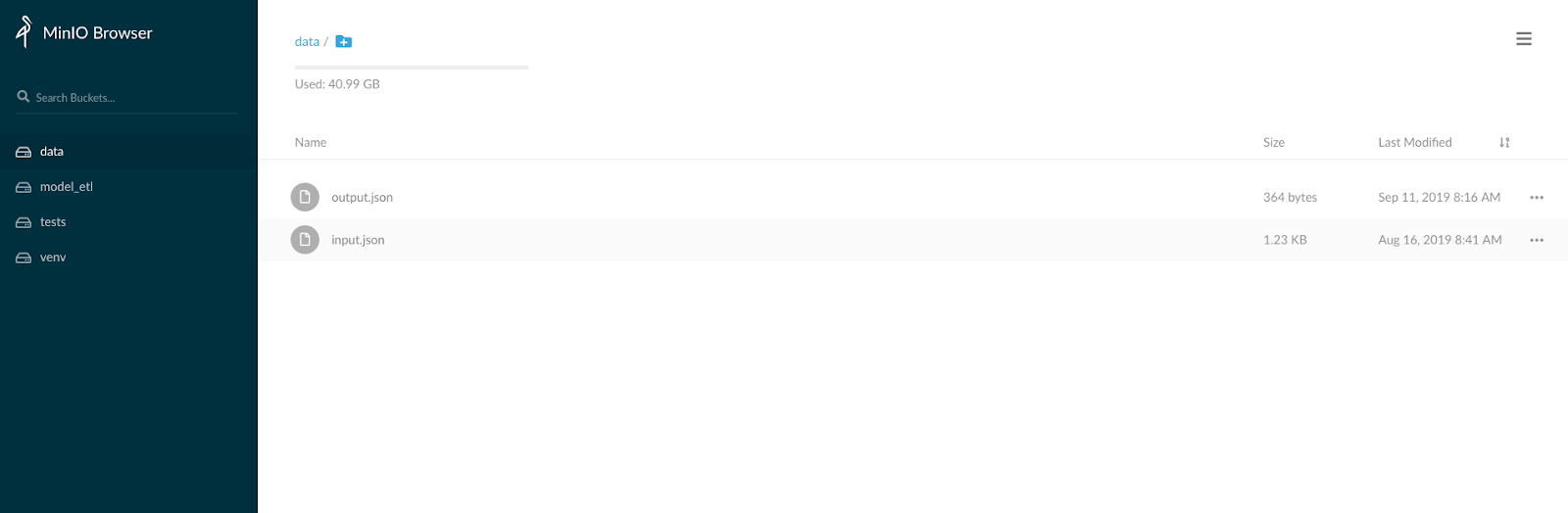
Now we can try out the new ETL job by executing this command:
export PYTHONPATH="${PYTHONPATH}:./"
python model_etl/s3_etl_job.py --input_file=input.json --output_file=output.json --bucket=data --key=TEST --secret_key=ASDFGHJKL --endpoint_url=http://127.0.0.1:9000/
The command above will run the new ETL, providing it with the credentials it needs to access the S3 service. This section showed how by injecting dependencies into the bonobo Graph, we can change the way the ETL accesses data without having to change the code of the ETL itself.
Closing
In this blog post, I showed how to deploy the iris model developed in a previous blog post inside of an ETL application. By splitting the deployment code and the model code into separate packages, I'm able to reuse the model in many different types of deployments. By structuring the codebases in this way, I'm able to keep the machine learning code separate from the deployment code very effectively.
In addition, by creating the MLModelTransformer class that works with the bonobo package, we can leverage all of the tools that bonobo has for building ETL applications. For example, the bonobo package provides functionality to load data from CSV files, JSON files, and databases. Bonobo also makes it easy to extend its capabilities with custom code through its highly modular object-oriented design. It also enforces good coding practices by supporting service dependency injection and parametrization.
One downside of this example is that this ETL is not meant to handle large scale data processing since it can only run in a single computer. A better way to do data processing over data sets that don't fit in the memory of a single computer is to use Apache Spark. Another drawback of the Bonobo package is that it does not support joins and aggregations over the data, since it only allows each incoming record to be processed individually.
Even though the ETL applications is able to make predictions with the MLModelTransformer class, it is very common for business logic to also be needed in a real-world deployment of an ML model. For example, we might want to prevent the model from making a prediction in certain locales or jurisdictions for legal reasons. For the sake of simplicity, I didn't include any business logic in the DAG we defined. The business logic should not be packaged inside of the MLModel class. We can keep it separate by creating a separate transformer that implements the business logic and putting it in the DAG. This way, we can apply the business logic without mixing it with the machine learning code in the MLModel class.
Another common situation in a real-world deployment of an ML model is the need to keep track of the predictions made by the model outside of the results that are provided to the clients of the system. This is a special log that the model generates as it is operating. Some of the contents of the prediction log would be: the inputs used to make a prediction, internal data that the model generated as it was making a prediction, and the output sent back to the client system. This is a more advanced requirement of an ML model deployment that I may expand on in another blog post.