Health Checks for ML Model Deployments
In a previous blog post we showed how to create a RESTful model service for a machine learning model. In this blog post, we'll extend the model service API by adding health checks to it.
This blog post was written in a Jupyter notebook, some of the code and commands found in it reflect this.
All of the code for this blog post is in this github repository.
Introduction
Deploying machine learning models in RESTful services is a common way to make the model available for use within a software system. In general, RESTful services are the most common type of service deployed, since they are simple to build, have wide compatibility, and have lots of tooling available for them. In order to monitor the availability of the service, RESTful APIs often provide health check endpoints which make it easy for an outside system to verify that the service is up and running. A health check endpoint is a simple endpoint that can be called by a process manager to ascertain whether the application is running correctly. In this blog post we'll be working with Kubernetes so we'll focus on the health checks supported by Kubernetes.
There are several types of health check endpoints supported by Kubernetes: startup, readiness, and liveness health checks. Startup checks are used to check if an application has started. If the container has a startup check configured on it, Kubernetes will wait until the application has finished starting up before moving on with the process of making the application available to clients. Startup checks are useful for applications that take a while to startup. Startup checks are only called during application startup, once an application has finished starting up the startup check is not called again.
Readiness checks are used to check if a container is ready to start accepting requests. Once the application has finished starting up, Kubernetes uses the readiness check to make sure that the application is able to accept requests. Service readiness can change during the service lifecycle so the check is called continuously until the application is stopped.
Liveness checks are used to restart a pod if the application is not responding. They are are the simplest type of check to implement in the application because they should always succeed if the server process is running. Liveness checks are useful to detect if the application is in an unsafe state, if the liveness check fails the process manager needs to restart the application to get it out of the unsafe state. Liveness checks are also called continuously while the application is running.
In this blog post, we’ll be adding startup, readiness, and liveness checks to a RESTful model service that is hosting a machine learning model. We'll also build a model that requires health checks in order to be deployed correctly.
Getting Data
In order to train a model, we first need to have a dataset. We went into Kaggle and found a dataset that contained loan information. To make it easy to download the data, we installed the kaggle python package. Then we executed these commands to download the data and unzip it into the data folder in the project:
from IPython.display import clear_output
!mkdir -p ../data

!kaggle datasets download -d ranadeep/credit-risk-dataset -p ../data --unzip

clear_output()
Let's look at the data files:
!ls -la ../data
total 67648
drwxr-xr-x 6 brian staff 192 Nov 21 14:45 [34m.[m[m
drwxr-xr-x 27 brian staff 864 Jan 11 21:23 [34m..[m[m
-rw-r--r--@ 1 brian staff 6148 Oct 31 17:30 .DS_Store
-rw-r--r-- 1 brian staff 20995 Nov 21 13:49 LCDataDictionary.xlsx
-rw-r--r-- 1 brian staff 34603008 Nov 21 14:58 credit-risk-dataset.zip
drwxr-xr-x 3 brian staff 96 Nov 16 09:33 [34mloan[m[m
Looks like the data is in a .csv file in the /loan folder and the data dictionary is in an excel spreadsheet file.
Let's load the data .csv file into a pandas dataframe.
import pandas as pd

data = pd.read_csv("../data/loan/loan.csv", low_memory=False)
data.info()
<class 'pandas.core.frame.DataFrame'>
RangeIndex: 887379 entries, 0 to 887378
Data columns (total 74 columns):
 #   Column                       Non-Null Count   Dtype
---  ------                       --------------   -----
 0   id                           887379 non-null  int64
 1   member_id                    887379 non-null  int64
 2   loan_amnt                    887379 non-null  float64
 3   funded_amnt                  887379 non-null  float64
 4   funded_amnt_inv              887379 non-null  float64
 5   term                         887379 non-null  object
 6   int_rate                     887379 non-null  float64
 7   installment                  887379 non-null  float64
 8   grade                        887379 non-null  object
 9   sub_grade                    887379 non-null  object
 10  emp_title                    835917 non-null  object
 11  emp_length                   842554 non-null  object
 12  home_ownership               887379 non-null  object
 13  annual_inc                   887375 non-null  float64
 14  verification_status          887379 non-null  object
 15  issue_d                      887379 non-null  object
 16  loan_status                  887379 non-null  object
 17  pymnt_plan                   887379 non-null  object
 18  url                          887379 non-null  object
 19  desc                         126028 non-null  object
 20  purpose                      887379 non-null  object
 21  title                        887227 non-null  object
 22  zip_code                     887379 non-null  object
 23  addr_state                   887379 non-null  object
 24  dti                          887379 non-null  float64
 25  delinq_2yrs                  887350 non-null  float64
 26  earliest_cr_line             887350 non-null  object
 27  inq_last_6mths               887350 non-null  float64
 28  mths_since_last_delinq       433067 non-null  float64
 29  mths_since_last_record       137053 non-null  float64
 30  open_acc                     887350 non-null  float64
 31  pub_rec                      887350 non-null  float64
 32  revol_bal                    887379 non-null  float64
 33  revol_util                   886877 non-null  float64
 34  total_acc                    887350 non-null  float64
 35  initial_list_status          887379 non-null  object
 36  out_prncp                    887379 non-null  float64
 37  out_prncp_inv                887379 non-null  float64
 38  total_pymnt                  887379 non-null  float64
 39  total_pymnt_inv              887379 non-null  float64
 40  total_rec_prncp              887379 non-null  float64
 41  total_rec_int                887379 non-null  float64
 42  total_rec_late_fee           887379 non-null  float64
 43  recoveries                   887379 non-null  float64
 44  collection_recovery_fee      887379 non-null  float64
 45  last_pymnt_d                 869720 non-null  object
 46  last_pymnt_amnt              887379 non-null  float64
 47  next_pymnt_d                 634408 non-null  object
 48  last_credit_pull_d           887326 non-null  object
 49  collections_12_mths_ex_med   887234 non-null  float64
 50  mths_since_last_major_derog  221703 non-null  float64
 51  policy_code                  887379 non-null  float64
 52  application_type             887379 non-null  object
 53  annual_inc_joint             511 non-null     float64
 54  dti_joint                    509 non-null     float64
 55  verification_status_joint    511 non-null     object
 56  acc_now_delinq               887350 non-null  float64
 57  tot_coll_amt                 817103 non-null  float64
 58  tot_cur_bal                  817103 non-null  float64
 59  open_acc_6m                  21372 non-null   float64
 60  open_il_6m                   21372 non-null   float64
 61  open_il_12m                  21372 non-null   float64
 62  open_il_24m                  21372 non-null   float64
 63  mths_since_rcnt_il           20810 non-null   float64
 64  total_bal_il                 21372 non-null   float64
 65  il_util                      18617 non-null   float64
 66  open_rv_12m                  21372 non-null   float64
 67  open_rv_24m                  21372 non-null   float64
 68  max_bal_bc                   21372 non-null   float64
 69  all_util                     21372 non-null   float64
 70  total_rev_hi_lim             817103 non-null  float64
 71  inq_fi                       21372 non-null   float64
 72  total_cu_tl                  21372 non-null   float64
 73  inq_last_12m                 21372 non-null   float64
dtypes: float64(49), int64(2), object(23)
memory usage: 501.0+ MB
We'll be predicting credit risk. Let's select the most promising columns in the dataset so that we wont have to deal with all of the columns.
data = data[[
    "annual_inc",
    "collections_12_mths_ex_med",
    "delinq_2yrs",
    "dti",
    "emp_length",
    "home_ownership",
    "acc_now_delinq",
    "installment",
    "int_rate",
    "last_pymnt_amnt",
    "loan_amnt",
    "loan_status",
    "pub_rec",
    "purpose",
    "revol_util",
    "term",
    "total_pymnt_inv",
    "verification_status"
]]
To make the data easier to explore we'll rename the columns to make their names more user friendly.
data = data.rename(columns={
    "annual_inc": "AnnualIncome",
    "collections_12_mths_ex_med": "CollectionsInLast12Months",
    "delinq_2yrs": "DelinquenciesInLast2Years",
    "dti": "DebtToIncomeRatio",
    "emp_length": "EmploymentLength",
    "home_ownership": "HomeOwnership",
    "acc_now_delinq": "NumberOfDelinquentAccounts",
    "installment": "MonthlyInstallmentPayment",
    "int_rate": "InterestRate",
    "last_pymnt_amnt": "LastPaymentAmount",
    "loan_amnt": "LoanAmount",
    "loan_status": "LoanStatus",
    "pub_rec": "DerogatoryPublicRecordCount",
    "purpose": "LoanPurpose",
    "revol_util": "RevolvingLineUtilizationRate",
    "term": "Term",
    "total_pymnt_inv": "TotalPaymentsToDate",
    "verification_status": "VerificationStatus",
})
We'll also build a simple data dictionary with the column descriptions that were downloaded with the dataset.
data_dictionary = {
    "AnnualIncome": "The self-reported annual income provided by the borrower during registration.",
    "CollectionsInLast12Months": "Number of collections in 12 months excluding medical collections.",
    "DelinquenciesInLast2Years": "The number of 30+ days past-due incidences of delinquency in the borrower's credit file for the past 2 years.",
    "DebtToIncomeRatio": "A ratio calculated using the borrower’s total monthly debt payments on the total debt obligations, excluding mortgage and the requested LC loan, divided by the borrower’s self-reported monthly income.",
    "EmploymentLength": "Employment length in years. Possible values are between 0 and 10 where 0 means less than one year and 10 means ten or more years.",
    "HomeOwnership": "The home ownership status provided by the borrower during registration. Our values are: RENT, OWN, MORTGAGE, OTHER.",
    "NumberOfDelinquentAccounts": "The number of accounts on which the borrower is now delinquent.",
    "MonthlyInstallmentPayment": "The monthly payment owed by the borrower if the loan originates.",
    "InterestRate": "Interest Rate on the loan.",
    "LastPaymentAmount": "Last total payment amount received.",
    "LoanAmount": "The listed amount of the loan applied for by the borrower.",
    "LoanStatus": "Current status of the loan.",
    "DerogatoryPublicRecordCount": "Number of derogatory public records.",
    "LoanPurpose": "A category provided by the borrower for the loan request.",
    "RevolvingLineUtilizationRate": "Revolving line utilization rate, or the amount of credit the borrower is using relative to all available revolving credit.",
    "Term": "The number of payments on the loan. Values are in months and can be either 36 or 60.",
    "TotalPaymentsToDate": "Payments received to date for portion of total amount funded by investors.",
    "VerificationStatus": "Indicates if income was verified.",
}
Building a Model
Now that we have the dataset, we'll start working on training a model. We'll be doing data exploration, data preparation, model training, and model validation.
Profiling the Data
Profiling the data can tell us a lot about the internal structure of the dataset. To profile the data, we'll use the pandas_profiling package.
To install the package, we'll execute this command:
!pip install pandas_profiling

clear_output()
The profile is built with this code:
from pandas_profiling import ProfileReport

profile = ProfileReport(data,
                        title="Credit Risk Analysis Dataset Report",
                        pool_size=4,
                        progress_bar=False,
                        dataset={
                            "description": "Lending Club loan data, complete loan data for all loans issued through the 2007-2015."
                        },
                        variables={
                            "descriptions": data_dictionary
                        })
We passed the data dictionary we built to the profile, it will be saved in the report generated.
Once the report is created, we'll save it to disk as an HTML file.
profile.to_file("../credit_risk_model/model_files/data_exploration_report.html")

clear_output()
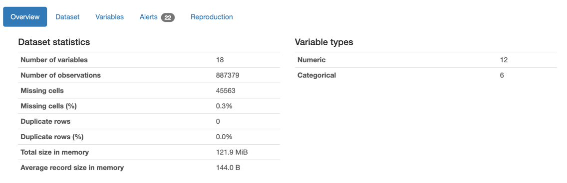
Right away the profile will tell us a few key details about the dataset:
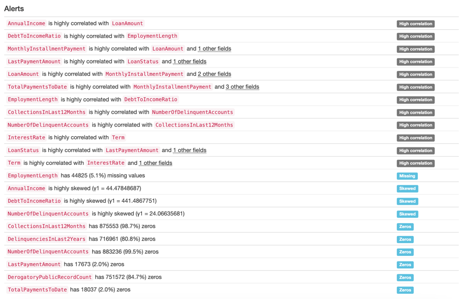
The profile also contains a few alerts about the data:
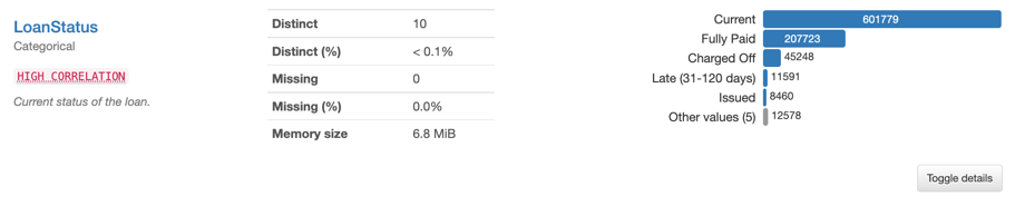
The profile has a description for each variable. Here's the description for the "LoanStatus" variable, which we will use to build the target variable.
By using the pandas_profiling package we can avoid writing the most common data analysis code that we write for all datasets.
Preparing the Data
The column that we're interested in is the "LoanStatus" column which tells us the current status of the loan. The values in the column are:
list(data["LoanStatus"].unique())
['Fully Paid',
 'Charged Off',
 'Current',
 'Default',
 'Late (31-120 days)',
 'In Grace Period',
 'Late (16-30 days)',
 'Does not meet the credit policy. Status:Fully Paid',
 'Does not meet the credit policy. Status:Charged Off',
 'Issued']
We'll be using this column to predict how risky a loan is. To do this, we'll need to create a target column that maps the values above into values that represent the riskiness of the loan. To keep things simple we'll simply create two categories for loans:
- "safe", for all loans that are current, fully paid off, in grace period, or the payment plan has not started yet
- "risky", for all other loans
Now we'll map the values above to the categories we want:
data["LoanRisk"] = data["LoanStatus"].replace({
    "Fully Paid": "safe",
    "Charged Off": "risky",
    "Current": "safe",
    "Default": "risky",
    "Late (31-120 days)": "risky",
    "In Grace Period": "safe",
    "Late (16-30 days)": "risky",
    "Does not meet the credit policy. Status:Fully Paid": "safe",
    "Does not meet the credit policy. Status:Charged Off": "risky",
    "Issued": "safe"
})

data.shape
(887379, 19)
Now we can remove the "LoanStatus" column since we created a new target column.
data = data.drop("LoanStatus", axis=1)

data.shape
(887379, 18)
Now that have a defined target column, we can move on to fixing some things in the dataset. From the profile we can see that there are several problems with the data that we need to fix.
The profile tells us that there are rows with missing data. To simplify the data modeling, we'll drop these rows.
data = data.dropna()

data.shape
(841954, 18)
All of the rows with missing values are now gone.
The "AnnualIncome" column is highly skewed. This is due to some rows which have outlier values, for example the max value for this column is $9,500,000. We'll fix this by removing rows with outlier values in that column. We'll remove the rows with values in this column that are more than three standard deviations from the mean like this:
import numpy as np
from scipy import stats

data = data[(np.abs(stats.zscore(data["AnnualIncome"])) < 3)]

data.shape
(835167, 18)
Another column in the dataset that is highly skewed is "DebtToIncomeRatio". For example, the maximum value in this column is 9999 which is probably not correct since most of the values in the column have a range between 0 and 100.
We'll use the same code to remove the outlier values for DebtToIncomeRatio.
data = data[(np.abs(stats.zscore(data["DebtToIncomeRatio"])) < 3)]

data.shape
(835112, 18)
The column "NumberOfDelinquentAccounts" is highly skewed because of a single record that has a value of 14. We'll remove the outliers by simply filtering out the rows with values above 6.
data = data[data["NumberOfDelinquentAccounts"] <= 6]

data.shape
(835111, 18)
The "HomeOwnership" column has several values that stand in for missing data. These values make up a small portion of the dataset, so we'll just remove the rows instead of doing data imputation.
data = data[data["HomeOwnership"] != "OTHER"]
data = data[data["HomeOwnership"] != "NONE"]
data = data[data["HomeOwnership"] != "ANY"]

data.shape
(834889, 18)
Looks like we only lost a few hundred rows from the dataset.
The variable "CollectionsInLast12Months" is not highly skewed but it contains values that only appear once or very few times. There are very few samples that have a value above 5, these samples are likely not useful so we'll remove them.
data = data[data["CollectionsInLast12Months"] <= 5]

data.shape
(834884, 18)
The same is true for the "DelinquenciesInLast2Years" and "DerogatoryPublicRecordCount" variables. There are very few samples with a value above 10 for these variables. We'll remove those samples.
data = data[data["DelinquenciesInLast2Years"] <= 10]
data = data[data["DerogatoryPublicRecordCount"] <= 10]

data.shape
(834415, 18)
The variable "RevolvingLineUtilizationRate" is a percent whose values must be between 0 and 100. There really isn't a way to use more than 100% of your revolving line of credit. However, this variable has values above 100, we'll remove those samples because they're bad data.
data = data[data["RevolvingLineUtilizationRate"] <= 100.0]

data.shape
(831103, 18)
Validating the Data
Next, we'll use the deepchecks package to do ML specific checks on the data. These checks are for checking for data issues that might affect an ML model.
Let's install the package:
!pip install deepchecks

clear_output()
Before we can run these checks, we need to specify which variables are categorical and numerical, and which variable is the target variable. We'll create lists of variable names for this purpose.
categorical_variables = [
    "EmploymentLength",
    "HomeOwnership",
    "LoanPurpose",
    "VerificationStatus",
    "Term"
]

numerical_variables = [
    "AnnualIncome",
    "CollectionsInLast12Months",
    "DelinquenciesInLast2Years",
    "DebtToIncomeRatio",
    "NumberOfDelinquentAccounts",
    "MonthlyInstallmentPayment",
    "InterestRate",
    "LastPaymentAmount",
    "LoanAmount",
    "DerogatoryPublicRecordCount",
    "RevolvingLineUtilizationRate",
    "TotalPaymentsToDate"
]

target_variable = "LoanRisk"

all_variables = categorical_variables + numerical_variables + [target_variable]

assert len(all_variables) == len(data.columns), "A column is missing from the lists of variables."
The assert statement at the end of the code above is a simple check that makes sure that we don't forget to include all of the columns in the lists. If we forget to include a column in the list it will stop execution of the notebook with an error message.
In order to avoid some errors in the training process, we'll need to change the column type of some of the columns in the pandas dataframe to "category".
for column_name in categorical_variables:
    data[column_name] = data[column_name].astype("category")
Lets start the data validation checks.
from deepchecks.tabular import Dataset
from deepchecks.tabular.suites import data_integrity

dataset = Dataset(data,
                  cat_features=categorical_variables,
                  label=target_variable)

clear_output()
The Dataset object contains a reference to the original Dataframe that we've been working with, and also contains the metadata about the columns in the dataframe that is needed to analyze the data.
We'll run the checks on the data like this:
data_integrity_suite = data_integrity()

suite_result = data_integrity_suite.run(dataset)

clear_output()
suite_result.save_as_html("../credit_risk_model/model_files/deepchecks_data_integrity_results.html")
'../credit_risk_model/model_files/deepchecks_data_integrity_results.html'
The checks done by this suite are geared towards datasets used for machine learning.
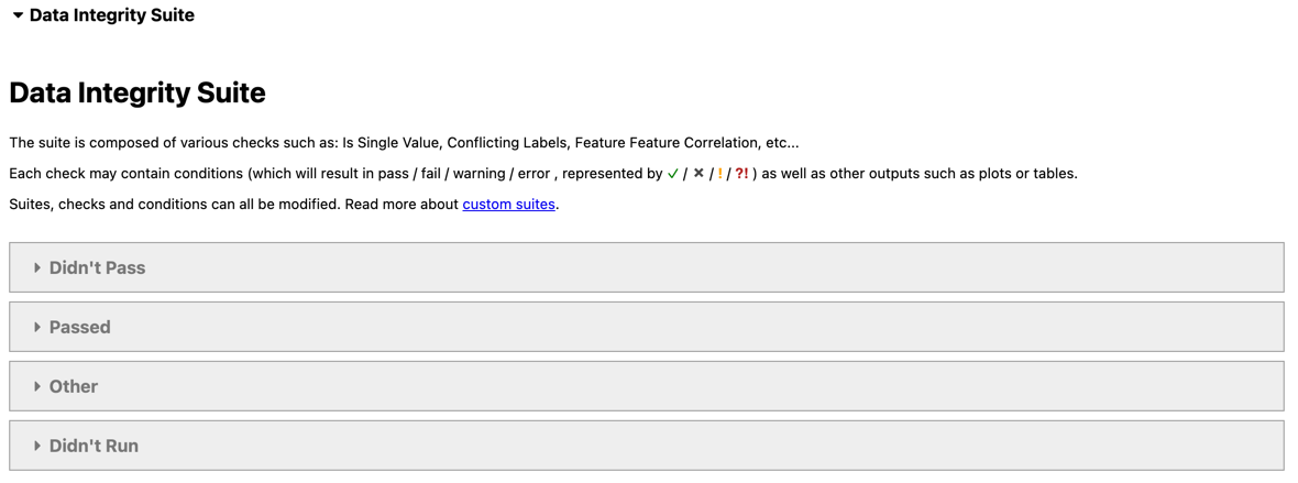
The results of the data integrity suite look like this:
The suite contains many checks that execute on the data set, the checks that passed are:
- Feature Label Correlation, predictive power score is less than 0.8 for all features.
- Single Value in Column, column does not contain only a single value
- Special Characters, ratio of samples containing solely special character is less or equal to 0.1%
- Mixed Nulls, number of different null types is less or equal to 1
- Mixed Data Types, rare data types in column are either more than 10% or less than 1% of the data
- Data Duplicates, duplicate data ratio is less or equal to 0%
- String Length Out Of Bounds, ratio of string length outliers is less or equal to 0%
- Conflicting Labels, ambiguous sample ratio is less or equal to 0%
The checks are fully explained in the deepchecks documentation.
For now, we're more interested in the checks that did not pass:
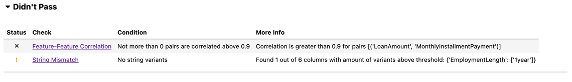
The two checks that didn't pass are:
- Feature-Feature Correlation, not more than 0 pairs are correlated above 0.9
- String Mismatch, no string variants
The deepchecks package found that the "LoanAmount" and "MonthlyInstallmentPayment" variables are highly correlated, which makes sense because an increase in loan amount will always cause an increase in payment amount. We can safely drop the MonthlyInstallmentPayment column from the dataset.
data = data.drop("MonthlyInstallmentPayment", axis=1)

numerical_variables.remove("MonthlyInstallmentPayment")

data.shape
(831103, 17)
The deepchecks package also found that the "EmploymentLength" variable contains string values that are similar to each other. For example, two levels found in the categorical variable are "1 year" and "< 1 year". This is a warning that we can ignore because the levels are correctly set.
We're now getting closer to a dataset that we can use to train a model . We'll be using deepchecks to do train/test dataset checks and model checks later on.
Training a Model
To train a model, we'll first create a training and testing set. We'll use 80% of the rows for training and 20% of the rows for testing.
import numpy as np

mask = np.random.rand(len(data)) < 0.80
training_data = data[mask]
testing_data = data[~mask]

print(training_data.shape)
print(testing_data.shape)
(664983, 17)
(166120, 17)
We will be running a test suite on the newly created training and test suites using deepchecks. The deepchecks package requires that we create two Dataset objects, one for the training set and one for the testing set.
train_dataset = Dataset(training_data,
                        label=target_variable,
                        cat_features=categorical_variables)

test_dataset = Dataset(testing_data,
                       label=target_variable,
                       cat_features=categorical_variables)
Now we can run the train-test validation suite.
from deepchecks.tabular.suites import train_test_validation

validation_suite = train_test_validation()

suite_result = validation_suite.run(train_dataset, test_dataset)

clear_output()
We'll save the results to files for this suite as well.
suite_result.save_as_html("../credit_risk_model/model_files/deepchecks_train_test_results.html")
'../credit_risk_model/model_files/deepchecks_train_test_results.html'
The results of the suite look like this:
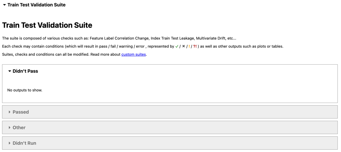
All of the checks in this suite passed:
- Datasets Size Comparison, Test-Train size ratio is greater than 0.01
- Category Mismatch Train Test, ratio of samples with a new category is less or equal to 0%
- Feature Label Correlation Change, Train-Test features' Predictive Power Score difference is less than 0.2
- Feature Label Correlation Change, Train features' Predictive Power Score is less than 0.7
- Train Test Feature Drift, categorical drift score < 0.2 and numerical drift score < 0.1
- Train Test Label Drift, categorical drift score < 0.2 and numerical drift score < 0.1 for label drift Label's drift score Cramer's V is 0
- New Label Train Test, number of new label values is less or equal to 0
- String Mismatch Comparison No new variants allowed in test data
- Train Test Samples Mix, percentage of test data samples that appear in train data is less or equal to 10%,
- Multivariate Drift, drift value is less than 0.25
These checks are more fully explained in the documentation.
Now that we have verified the contents of the training and testing sets, we're finally ready to traing a model. To do this, we'll need to create separate dataframes for the predictor and target columns:
feature_columns = categorical_variables + numerical_variables

X_train = training_data[feature_columns]
y_train = training_data[target_variable]

X_test = testing_data[feature_columns]
y_test = testing_data[target_variable]
We'll be using the LightGBM package to train a GBM model and the FLAML package for doing automated machine learning. Let's install the packages:
!pip install lightgbm
!pip install flaml

clear_output()
Let's train a model using the default hyperparameters to have a baseline.
%%time
from lightgbm import LGBMClassifier

model = LGBMClassifier()

model = model.fit(X_train, y_train)
CPU times: user 13.1 s, sys: 657 ms, total: 13.8 s
Wall time: 3.46 s
Now let's calculate the classification metrics for this simple model:
%%time
from sklearn.metrics import classification_report

y_pred = model.predict(X_test)

print(classification_report(y_test, y_pred))
              precision    recall  f1-score   support

       risky       0.92      0.14      0.24     11456
        safe       0.94      1.00      0.97    154664

    accuracy                           0.94    166120
   macro avg       0.93      0.57      0.61    166120
weighted avg       0.94      0.94      0.92    166120

CPU times: user 8.96 s, sys: 191 ms, total: 9.15 s
Wall time: 6.52 s
The "safe" class has good metrics but the "risky" class does not. This is due to the fact that the classes are imbalanced.
We'll try to fix this issue by doing automated ML with the FLAML package. The automated hyperparameter search will hopefully find some parameters that can improve the metrics of the "risky" class.
The settings are:
- time_budget: amount of time allowed for the auto ML algorithm to run
- metric: the metric that should be maximized by the auto ML alogorithm
- estimator_list: the types of estimators that can be used by FLAML, in this case we only want to try LightGBM
- task: the type of task that the estimator should be solving
- log_file_name: name of the log file output by the auto ML algorithm
- seed: the random seed to be used by the auto ML algorithm
from flaml import AutoML

automl = AutoML()

settings = {
    "time_budget": 1200,
    "metric": "roc_auc",
    "estimator_list": ["lgbm"],
    "task": "classification",
    "log_file_name": "experiment.log",
    "seed": 42
}

automl.fit(X_train=X_train, y_train=y_train, **settings)

clear_output()
The hyperparameter search has found an optimal set of hyperparametes using the training set and cross validation. These are the hyperparameters found:
automl.best_config
{'n_estimators': 10707,
 'num_leaves': 7,
 'min_child_samples': 62,
 'learning_rate': 0.24185440044608203,
 'log_max_bin': 10,
 'colsample_bytree': 0.9914098492087268,
 'reg_alpha': 2.551067627605118,
 'reg_lambda': 0.0010846951681516895}
Let's train a model using the optimal hyperparameters:
model = LGBMClassifier(**automl.best_config)

model = model.fit(X_train, y_train)
Let's get the the classification metrics for the best model:
y_pred = model.predict(X_test)

print(classification_report(y_test, y_pred))
              precision    recall  f1-score   support

       risky       0.89      0.46      0.61     11456
        safe       0.96      1.00      0.98    154664

    accuracy                           0.96    166120
   macro avg       0.93      0.73      0.79    166120
weighted avg       0.96      0.96      0.95    166120
Validating the Model
Deepchecks is also able to validate the model with the model_evaluation suite of checks.
from deepchecks.tabular.suites import model_evaluation

evaluation_suite = model_evaluation()

suite_result = evaluation_suite.run(train_dataset, test_dataset, model)
suite_result.save_as_html("../credit_risk_model/model_files/deepchecks_model_evaluation_results.html")
'../credit_risk_model/model_files/deepchecks_model_evaluation_results.html'
Packaging the Model Files
Let's serialize the best model to disk:
%%time
import joblib

joblib.dump(model, "../credit_risk_model/model_files/model.joblib")
CPU times: user 1.33 s, sys: 82.1 ms, total: 1.41 s
Wall time: 226 ms


['../credit_risk_model/model_files/model.joblib']
!ls -la ../credit_risk_model/model_files
total 82824
drwxr-xr-x 8 brian staff 256 Jan 15 20:07 [34m.[m[m
drwxr-xr-x 8 brian staff 256 Dec 13 11:15 [34m..[m[m
-rw-r--r--@ 1 brian staff 6148 Jan 15 19:09 .DS_Store
-rw-r--r-- 1 brian staff 9426966 Jan 15 19:12 data_exploration_report.html
-rw-r--r-- 1 brian staff 7750291 Jan 15 19:15 deepchecks_data_integrity_results.html
-rw-r--r--@ 1 brian staff 7964754 Jan 15 20:06 deepchecks_model_evaluation_results.html
-rw-r--r-- 1 brian staff 7793791 Jan 15 19:17 deepchecks_train_test_results.html
-rw-r--r-- 1 brian staff 9452707 Jan 15 20:07 model.joblib
The serialized model is 9.5 megabytes in size and took 226 milliseconds to write to disk. This is important to note because we will need to deserialize the model later in order to make predictions with it.
In the process of training this model, we created a few files. To be able to use these files later, we'll package them up and save them in a location that can be accessed by the prediction code later. We'll be using a .zip file for this purpose.
import shutil


shutil.make_archive("../credit_risk_model/model_files/1", "zip", "../credit_risk_model/model_files")
'/Users/brian/Code/health-checks-for-ml-model-deployments/credit_risk_model/model_files/1.zip'
The command created a .zip file with all of the files in the model_files folder. The name of the folder is "1.zip" this is just a simple name that denotes that it is the first model trained for the credit_risk_model package.
Now that we have the model files in a .zip file, we can delete the original files from the folder:
!rm ../credit_risk_model/model_files/data_exploration_report.html
!rm ../credit_risk_model/model_files/deepchecks_data_integrity_results.html
!rm ../credit_risk_model/model_files/deepchecks_train_test_results.html
!rm ../credit_risk_model/model_files/deepchecks_model_evaluation_results.html
!rm ../credit_risk_model/model_files/model.joblib
This packaging process ensures that all of the results of the model training process end up in one archive that we can use later. All of the data and model check results are packaged along with the serialized model so its easy to review the model training process.
Making Predictions with the Model
We now have a working model that accepts Pandas dataframes as input and also returns predictions in dataframes. This is useful in the context of model training, but makes integrating the model with other software components a lot more complicated. To make the model easier to use, we'll need to create input and output schemas for the model and also create a wrapper class that provides a consistent interface for the model.
We'll create the model's input and output schemas with the pydantic package, which is a package used for data validation. By creating the schemas using this package we're able to fully document the inputs that the model accepts and the expected outputs of the model we're going to deploy.
To begin, we'll define the allowed values for the categorical variables.
from pydantic import BaseModel, Field
from enum import Enum


class EmploymentLength(str, Enum):
    """Employment length in years."""
    less_than_1_year = "< 1 year"
    one_year = "1 year"
    two_years = "2 years"
    three_years = "3 years"
    four_years = "4 years"
    five_years = "5 years"
    six_years = "6 years"
    seven_years = "7 years"
    eight_years = "8 years"
    nine_years = "9 years"
    ten_years_or_more = "10+ years"


class HomeOwnership(str, Enum):
    """The home ownership status provided by the borrower during registration."""
    MORTGAGE = "MORTGAGE"
    RENT = "RENT"
    OWN = "OWN"


class LoanPurpose(str, Enum):
    """A category provided by the borrower for the loan request."""
    debt_consolidation = "debt_consolidation"
    credit_card = "credit_card"
    home_improvement = "home_improvement"
    other = "other"
    major_purchase = "major_purchase"
    small_business = "small_business"
    car = "car"
    medical = "medical"
    moving = "moving"
    vacation = "vacation"
    wedding = "wedding"
    house = "house"
    renewable_energy = "renewable_energy"
    educational = "educational"


class Term(str, Enum):
    """The number of payments on the loan."""
    thirty_six_months = " 36 months"
    sixty_months = " 60 months"


class VerificationStatus(str, Enum):
    """Indicates if income was verified."""
    source_verified = "Source Verified"
    verified = "Verified"
    not_verified = "Not Verified"
The dataset contains 5 categorical variables, so we defined 5 Enum classes that contain the values accepted for these variables. Each enumeration has a key and value, with the value being the value as the model expects to see it. By using enumerated values, we can ensure that the model can only receive values in these inputs that it has previously seen in the training set.
Now that we have the categorical variables defined, we can define the input schema for the model:
class CreditRiskModelInput(BaseModel):
    """Inputs for predicting credit risk."""
    annual_income: int = Field(ge=1896, le=273000, description="The self-reported annual income provided by the borrower during registration.")
    collections_in_last_12_months: int = Field(ge=0, le=20, description="Number of collections in 12 months excluding medical collections.")
    delinquencies_in_last_2_years: int = Field(ge=0, le=39, description="The number of 30+ days past-due incidences of delinquency in the borrower's credit file for the past 2 years.")
    debt_to_income_ratio: float = Field(ge=0.0, le=42.64, description="A ratio calculated using the borrower’s total monthly debt payments on the total debt obligations, excluding mortgage and the requested LC loan, divided by the borrower’s self-reported monthly income.")
    employment_length: EmploymentLength = Field(description="Employment length in years.")
    home_ownership: HomeOwnership = Field(description="The home ownership status provided by the borrower during registration. Our values are: RENT, OWN, MORTGAGE, OTHER.")
    number_of_delinquent_accounts: int = Field(ge=0, le=6, description="The number of accounts on which the borrower is now delinquent.")
    interest_rate: float = Field(ge=5.32, le=28.99, description="Interest Rate on the loan.")
    last_payment_amount: float = Field(ge=0.0, le=36475.59, description="Last total payment amount received.")
    loan_amount: int = Field(ge=500.0, le=35000.0, description="The listed amount of the loan applied for by the borrower.")
    derogatory_public_record_count: int = Field(ge=0.0, le=86.0, description="Number of derogatory public records.")
    loan_purpose: LoanPurpose = Field(description="A category provided by the borrower for the loan request.")
    revolving_line_utilization_rate: float = Field(ge=0.0, le=892.3, description="Revolving line utilization rate, or the amount of credit the borrower is using relative to all available revolving credit.")
    term: Term = Field(description="The number of payments on the loan. Values are in months and can be either 36 or 60.")
    total_payments_to_date: float = Field(ge=0.0, le=57777.58, description="Payments received to date for portion of total amount funded by investors.")
    verification_status: VerificationStatus = Field(description="Indicates if income was verified.")
The schema is called "CreditRiskModelInput" and contains fields for each variable found in the dataset. We're using the Enum classes we defined above for the categorical fields, and we defined fields for all of the numerical variables. Each numerical field has a range of allowed values that matches the range of the numerical variable found in the dataset. Each field also has a description of the variable that helps the user of the model to correctly feed data to the model.
The process of creating an input data schema makes the model much more used friendly and exposes information found in the dataset that the model was originally trained on to the user of the model. Doing this also allows us to build documentation for the model service automatically.
Now that we have the model's input schema defined, we'll define the output schema:
class CreditRisk(str, Enum):
    """Indicates whether or not loan is risky."""
    safe = "safe"
    risky = "risky"


class CreditRiskModelOutput(BaseModel):
    credit_risk: CreditRisk = Field(description="Whether or not the loan is risky.")
The model is a classification model and the output schema simply enumerates the classes that the model can predict.
We now have the input and output schemas defined, now we can tie it all together by creating a wrapper class for the model. The ml_base package defines a simple base class for model prediction code that allows us to "wrap" the prediction code in a class that follows the MLModel interface. This interface publishes this information about the model:
- Qualified Name, a unique identifier for the model
- Display Name, a friendly name for the model used in user interfaces
- Description, a description for the model
- Version, semantic version of the model codebase
- Input Schema, an object that describes the model\'s input data
- Output Schema, an object that describes the model\'s output schema
The MLModel interface also dictates that the model class implements two methods:
- __init__, the initialization method which loads any model artifacts needed to make predictions
- predict, prediction method that receives model inputs makes a prediction and returns model outputs
By using the MLModel base class we'll be able to do more interesting things later with the model. If you'd like to learn more about the ml_base package, here is some documentation about it.
To install the ml_base package, execute this command:
!pip install ml_base

clear_output()
We'll define the wrapper class like this:
import sys
import os
import joblib
import pandas as pd
from ml_base import MLModel
import zipfile


__file__ = os.path.join(os.path.dirname(os.path.realpath(os.path.abspath(''))), "credit_risk_model", "prediction", "model.py")

class CreditRiskModel(MLModel):
    """Prediction logic for the Credit Risk Model."""

    @property
    def display_name(self) -> str:
        """Return display name of model."""
        return "Credit Risk Model"

    @property
    def qualified_name(self) -> str:
        """Return qualified name of model."""
        return "credit_risk_model"

    @property
    def description(self) -> str:
        """Return description of model."""
        return "Model to predict the credit risk of a loan."

    @property
    def version(self) -> str:
        """Return version of model."""
        return "0.1.0"

    @property
    def input_schema(self):
        """Return input schema of model."""
        return CreditRiskModelInput

    @property
    def output_schema(self):
        """Return output schema of model."""
        return CreditRiskModelOutput

    def __init__(self):
        """Class constructor that loads and deserializes the model parameters."""
        dir_path = os.path.dirname(os.path.dirname(os.path.realpath(__file__)))
        file_path = os.path.join(dir_path, "model_files", "1.zip")

        with zipfile.ZipFile(file_path) as zf:
            if "model.joblib" not in zf.namelist():
                raise ValueError("Could not find model file in zip file.")
            model_file = zf.open("model.joblib")
            self._model = joblib.load(model_file)

    def predict(self, data: CreditRiskModelInput) -> CreditRiskModelOutput:
        """Make a prediction with the model.

        Params:
            data: Data for making a prediction with the model.

        Returns:
            The result of the prediction.

        """
        if type(data) is not CreditRiskModelInput:
            raise ValueError("Input must be of type 'CreditRisk'")

        X = pd.DataFrame([[
            data.employment_length.value,
            data.home_ownership.value,
            data.loan_purpose.value,
            data.verification_status.value,
            data.term.value,
            data.annual_income,
            data.collections_in_last_12_months,
            data.delinquencies_in_last_2_years,
            data.debt_to_income_ratio,
            data.number_of_delinquent_accounts,
            data.interest_rate,
            data.last_payment_amount,
            data.loan_amount,
            data.derogatory_public_record_count,
            data.revolving_line_utilization_rate,
            data.total_payments_to_date,
        ]],
            columns=[
                "EmploymentLength",
                "HomeOwnership",
                "LoanPurpose",
                "VerificationStatus",
                "Term",
                "AnnualIncome",
                "CollectionsInLast12Months",
                "DelinquenciesInLast2Years",
                "DebtToIncomeRatio",
                "NumberOfDelinquentAccounts",
                "InterestRate",
                "LastPaymentAmount",
                "LoanAmount",
                "DerogatoryPublicRecordCount",
                "RevolvingLineUtilizationRate",
                "TotalPaymentsToDate"
            ])

        categorical_variables = ["EmploymentLength",
                                 "HomeOwnership",
                                 "LoanPurpose",
                                 "VerificationStatus",
                                 "Term"]

        for column_name in categorical_variables:
            X[column_name] = X[column_name].astype("category")

        y_hat = self._model.predict(X)[0]

        return CreditRiskModelOutput(credit_risk=CreditRisk[y_hat])
We can make a prediction with the model by first building a CreditRiskModelInput object:
model_input = CreditRiskModelInput(
    annual_income=273000,
    collections_in_last_12_months=20,
    delinquencies_in_last_2_years=39,
    debt_to_income_ratio=42.64,
    employment_length=EmploymentLength.less_than_1_year,
    home_ownership=HomeOwnership.MORTGAGE,
    number_of_delinquent_accounts=6,
    interest_rate=28.99,
    last_payment_amount=36475.59,
    loan_amount=35000,
    derogatory_public_record_count=86,
    loan_purpose=LoanPurpose.debt_consolidation,
    revolving_line_utilization_rate=892.3,
    term=Term.thirty_six_months,
    total_payments_to_date=57777.58,
    verification_status=VerificationStatus.source_verified
)
Next, we'll instantiate the model class we defined above:
%%time
model = CreditRiskModel()
CPU times: user 372 ms, sys: 29.2 ms, total: 401 ms
Wall time: 113 ms
Notice that the model object took 113 milliseconds to be instantiated. This is because the model parameters take a lot of disk space and take a while to load from the hard drive. This is something that we'll need to deal with later.
We'll use the CreditRiskModelInput instance to make a prediction like this:
prediction = model.predict(model_input)

prediction
CreditRiskModelOutput(credit_risk=<CreditRisk.safe: 'safe'>)
The model predicted that the loan is "safe".
Creating a RESTful Service
Now that we have a model, we can deploy it in a service that allows clients to make predictions. To do this, we won't need to write any extra code, we can leverage the rest_model_service package to provide the RESTful API for the service. You can learn more about the package in this blog post.
To install the package, execute this command:
!pip install rest_model_service

clear_output()
To create a service for our model, all that is needed is that we add a YAML configuration file to the project. The configuration file looks like this:
service_title: Credit Risk Model Service
description: "Service hosting the Credit Risk Model."
version: "0.1.0"
models:
  - qualified_name: credit_risk_model
    class_path: credit_risk_model.prediction.model.CreditRiskModel
    create_endpoint: true
At the root of the YAML, the "service_title" field is the name of the service as it will appear in the documentation. The "description" and "version"fields will also be used to create the service documentation.
The models field is an array that contains the details of the models we would like to deploy in the service. The "qualified_name" field is the name we gave to the model. The "class_path" field points at the MLModel class that implements the model's prediction logic, in this case it is pointing to the class we built earlier in this blog post. The "create_endpoint" field tells the service to create an endpoint for the model.
Using the configuration file, we can create an OpenAPI specification file for the model service by executing these commands:
export PYTHONPATH=./
generate_openapi --configuration_file=./configuration/rest_configuration.yaml --output_file="service_contract.yaml"
The service_contract.yaml file is generated and contains the OpenAPI specification that was generated for the model service. The specification contains a description of the model's endpoint. The model's input and output schemas are automatically extracted and added to the specification. The OpenAPI specification file generated can be found at the root of the github repository in the file named service_contract.yaml
To run the service locally, execute these commands:
export REST_CONFIG=./configuration/rest_configuration.yaml
uvicorn rest_model_service.main:app
The service process starts up and can be accessed in a web browser at http://127.0.0.1:8000. The service renders the OpenAPI specification as a webpage that looks like this:
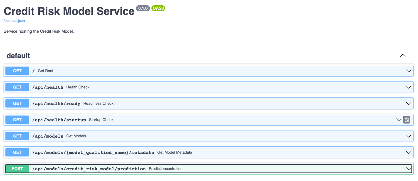
By using the MLModel base class provided by the ml_base package and the REST service framework provided by the rest_model_service package we're able to quickly stand up a service to host the model.
We can make a prediction using the model running in the service with this command:
!curl -X 'POST' \
  'http://127.0.0.1:8000/api/models/credit_risk_model/prediction' \
  -H 'accept: application/json' \
  -H 'Content-Type: application/json' \
  -d "{ \
      \"annual_income\": 273000, \
      \"collections_in_last_12_months\": 20, \
      \"delinquencies_in_last_2_years\": 39, \
      \"debt_to_income_ratio\": 42.64, \
      \"employment_length\": \"< 1 year\", \
      \"home_ownership\": \"MORTGAGE\", \
      \"number_of_delinquent_accounts\": 6, \
      \"interest_rate\": 28.99, \
      \"last_payment_amount\": 36475.59, \
      \"loan_amount\": 35000,  \
      \"derogatory_public_record_count\": 86, \
      \"loan_purpose\": \"debt_consolidation\", \
      \"revolving_line_utilization_rate\": 892.3, \
      \"term\": \" 36 months\", \
      \"total_payments_to_date\": 57777.58, \
      \"verification_status\": \"Source Verified\" \
}"
{"credit_risk":"safe"}
The model returned a prediction of "safe" for the loan.
Understanding Health Checks
The service is able exposes health information about itself through health endpoints. The health endpoints are:
- /api/health: indicates whether the service process is running. This endpoint will return a 200 status once the service has started.
- /api/health/ready: indicates whether the service is ready to respond to requests. This endpoint will return a 200 status only if all the models and decorators have finished being instantiated without errors.
- /api/health/startup: indicates whether the service is started. This endpoint will return a 200 status only if all the models and decorators have finished being instantiated without errors.
These endpoints are important for our use case because our model takes a while to load and become ready to be served over the API. The service will not be ready to serve traffic for a while, so the readiness and startup checks will fail until the models are ready.
The service is running so we'll try out each endpoint with a request:
!curl -X 'GET' \
  'http://127.0.0.1:8000/api/health' \
  -H 'accept: application/json'
{"health_status":"HEALTHY"}
The health endpoint returned a status of "HEALTHY".
!curl -X 'GET' \
  'http://127.0.0.1:8000/api/health/ready' \
  -H 'accept: application/json'
{"readiness_status":"ACCEPTING_TRAFFIC"}
The readiness status endpoint returned a status of "ACCEPTING_TRAFFIC".
!curl -X 'GET' \
  'http://127.0.0.1:8000/api/health/startup' \
  -H 'accept: application/json'
{"startup_status":"STARTED"}
The startup status endpoint returned a status of "STARTED".
During normal operation, the health endpoints are not very interesting. However, in special situations they are very useful. For example, if a model takes a long time to start up, the startup check endpoint will not return a 200 status response until each model is initiated and ready to make predictions. The readiness endpoint will also not return a 200 status until the model is ready. We'll use the healtcheck endpoints to integrated with Kubernetes.
Creating a Docker Image
Now that we have a working model and model service, we'll need to deploy it somewhere. We'll start by deploying the service locally using Docker.
Let's create a docker image and run it locally. The docker image is generated using instructions in the Dockerfile:
# syntax=docker/dockerfile:1
FROM python:3.9-slim

ARG BUILD_DATE

LABEL org.opencontainers.image.title="Health Checks for ML Models"
LABEL org.opencontainers.image.description="Health checks for ML models."
LABEL org.opencontainers.image.created=$BUILD_DATE
LABEL org.opencontainers.image.authors="6666331+schmidtbri@users.noreply.github.com"
LABEL org.opencontainers.image.source="https://github.com/schmidtbri/health-checks-for-ml-models"
LABEL org.opencontainers.image.version="0.1.0"
LABEL org.opencontainers.image.licenses="MIT License"
LABEL org.opencontainers.image.base.name="python:3.9-slim"

WORKDIR /service

ARG USERNAME=service-user
ARG USER_UID=10000
ARG USER_GID=10000

# install packages
RUN apt-get update \
    && apt-get install --assume-yes --no-install-recommends sudo \
    && apt-get install --assume-yes --no-install-recommends git \
    && apt-get install -y --no-install-recommends apt-utils \
    && apt-get install -y --no-install-recommends libgomp1 \
    && apt-get clean \
    && rm -rf /var/lib/apt/lists/*

# create a user
RUN groupadd --gid $USER_GID $USERNAME \
    && useradd --uid $USER_UID --gid $USER_GID -m $USERNAME \
    && echo $USERNAME ALL=\(root\) NOPASSWD:ALL > /etc/sudoers.d/$USERNAME \
    && chmod 0440 /etc/sudoers.d/$USERNAME

# installing dependencies
COPY ./service_requirements.txt ./service_requirements.txt
RUN pip install -r service_requirements.txt

# copying code and license
COPY ./credit_risk_model ./credit_risk_model
COPY ./LICENSE ./LICENSE

USER $USERNAME

CMD ["uvicorn", "rest_model_service.main:app", "--host", "0.0.0.0", "--port", "8000"]
The Dockerfile is used by this docker command to create a docker image:
!docker build -t credit_risk_model_service:0.1.0 ../

clear_output()
To make sure everything worked as expected, we'll look through the docker images in our system:
!docker image ls | grep credit_risk_model_service
credit_risk_model_service 0.1.0 fc3c3c747e2b 4 seconds ago 614MB
The credit_risk_model_service image is listed. Next, we'll start the image to see if the service is working correctly.
!docker run -d \
    -p 8000:8000 \
    -e REST_CONFIG=./configuration/rest_configuration.yaml \
    -v $(pwd)/../configuration:/service/configuration \
    --name credit_risk_model_service \
    credit_risk_model_service:0.1.0
706ff17d8db159568989d8a74221b8bc3bbcb52074ca61da1ee4015297035dc6
To make sure the server process started up correctly, we'll look at the logs:
!docker logs credit_risk_model_service
INFO:     Started server process [1]
INFO:     Waiting for application startup.
INFO:     Application startup complete.
INFO:     Uvicorn running on http://0.0.0.0:8000 (Press CTRL+C to quit)
The logs look good and the service is up and running.
The service should be accessible on port 8000 of localhost, so we'll try to make a prediction using the curl command:
!curl -X 'POST' \
  'http://127.0.0.1:8000/api/models/credit_risk_model/prediction' \
  -H 'accept: application/json' \
  -H 'Content-Type: application/json' \
  -d "{ \
      \"annual_income\": 273000, \
      \"collections_in_last_12_months\": 20, \
      \"delinquencies_in_last_2_years\": 39, \
      \"debt_to_income_ratio\": 42.64, \
      \"employment_length\": \"< 1 year\", \
      \"home_ownership\": \"MORTGAGE\", \
      \"number_of_delinquent_accounts\": 6, \
      \"interest_rate\": 28.99, \
      \"last_payment_amount\": 36475.59, \
      \"loan_amount\": 35000,  \
      \"derogatory_public_record_count\": 86, \
      \"loan_purpose\": \"debt_consolidation\", \
      \"revolving_line_utilization_rate\": 892.3, \
      \"term\": \" 36 months\", \
      \"total_payments_to_date\": 57777.58, \
      \"verification_status\": \"Source Verified\" \
}"
{"credit_risk":"safe"}
The model predicted that the loan is safe.
We're done with the docker container, so we'll shut down the model service container.
!docker kill credit_risk_model_service
!docker rm credit_risk_model_service
credit_risk_model_service
credit_risk_model_service
Creating a Kubernetes Cluster
To show the system in action, we’ll deploy the service to a Kubernetes cluster. A local cluster can be easily started by using minikube. Installation instructions can be found here.
To start the minikube cluster execute this command:
!minikube start
😄 minikube v1.28.0 on Darwin 13.0.1
✨ Using the docker driver based on existing profile
👍 Starting control plane node minikube in cluster minikube
🚜 Pulling base image ...
🔄 Restarting existing docker container for "minikube" ...
🐳 Preparing Kubernetes v1.25.3 on Docker 20.10.20 ...[K[K[K[K[K[K[K[K[K[K[K[K[K[K[K[K[K[K[K[K[K[K[K[K[K[K[K[K[K[K[K[K[K[K[K[K[K[K[K[K[K[K[K[K[K[K[K[K[K[K[K[K[K[K[K[K[K[K[K[K[K[K[K[K[K[K[K[K[K[K[K[K[K[K[K[K[K[K[K[K[K[K[K[K[K[K[K[K[K[K[K[K[K[K[K[K[K[K[K[K[K[K[K[K[K[K[K[K[K[K[K[K[K[K[K[K[K[K[K[K[K[K[K[K[K[K[K[K[K[K[K[K[K[K[K[K[K[K[K[K[K[K[K[K[K[K[K[K[K[K[K[K[K[K[K[K[K[K[K[K[K[K[K[K[K[K[K[K[K[K[K[K[K[K[K[K[K[K[K[K[K[K[K[K[K[K[K[K[K[K[K[K[K[K[K[K[K[K[K[K[K[K[K[K[K[K[K[K[K[K[K[K[K[K[K[K[K[K[K[K[K[K[K[K[K[K[K[K[K[K[K[K[K[K[K[K[K[K[K[K[K[K[K[K[K[K[K[K[K[K[K[K[K[K[K[K[K[K[K[K[K[K[K[K[K[K[K[K[K[K[K[K[K[K[K[K[K[K[K[K[K[K[K[K[K[K
🔎 Verifying Kubernetes components...
▪ Using image docker.io/kubernetesui/dashboard:v2.7.0
▪ Using image gcr.io/k8s-minikube/storage-provisioner:v5
▪ Using image docker.io/kubernetesui/metrics-scraper:v1.0.8
💡 Some dashboard features require the metrics-server addon. To enable all features please run:
minikube addons enable metrics-server
🌟 Enabled addons: storage-provisioner, default-storageclass, dashboard
🏄 Done! kubectl is now configured to use "minikube" cluster and "default" namespace by default
Let's view all of the pods running in the minikube cluster to make sure we can connect.
!kubectl get pods -A
NAMESPACE              NAME                                        READY   STATUS    RESTARTS         AGE
kube-system            coredns-565d847f94-2v6l9                    0/1     Running   10 (3d20h ago)   11d
kube-system            etcd-minikube                               0/1     Running   10 (3d20h ago)   11d
kube-system            kube-apiserver-minikube                     0/1     Running   10 (3d20h ago)   11d
kube-system            kube-controller-manager-minikube            0/1     Running   10 (25s ago)     11d
kube-system            kube-proxy-ztbgd                            1/1     Running   10 (25s ago)     11d
kube-system            kube-scheduler-minikube                     0/1     Running   10 (25s ago)     11d
kube-system            storage-provisioner                         1/1     Running   18 (25s ago)     11d
kubernetes-dashboard   dashboard-metrics-scraper-b74747df5-x559p   1/1     Running   9 (25s ago)      11d
kubernetes-dashboard   kubernetes-dashboard-57bbdc5f89-9jvln       1/1     Running   14 (3d20h ago)   11d
The pods running the kubernetes dashboard and other cluster services appear in the kube-system and kubernetes-dashboard namespaces.
Creating a Kubernetes Namespace
Now that we have a cluster and are connected to it, we'll create a namespace to hold the resources for our model deployment. The resource definition is in the kubernetes/namespace.yaml file. To apply the manifest to the cluster, execute this command:
!kubectl create -f ../kubernetes/namespace.yaml
namespace/model-services created
resourcequota/model-services-resource-quota created
The namespace was created, alongside with a ResourceQuota which limits the amount of resources that can be taken by objects within the namespace.
To take a look at the namespaces, execute this command:
!kubectl get namespace
NAME                   STATUS   AGE
default                Active   11d
kube-node-lease        Active   11d
kube-public            Active   11d
kube-system            Active   11d
kubernetes-dashboard   Active   11d
model-services         Active   0s
The new namespace appears in the listing along with other namespaces created by default by the system. To use the new namespace for the rest of the operations, execute this command:
!kubectl config set-context --current --namespace=model-services
Context "minikube" modified.
Creating a Kubernetes Deployment and Service
The model service is deployed by using Kubernetes resources. These are:
- Model Service ConfigMap: a set of configuration options, in this case it is a simple YAML file that will be loaded into the running container as a volume mount. This resource allows us to change the configuration of the model service without having to modify the Docker image. The configuration file will overwrite the configuration files that were included with the Docker image.
- Deployment: a declarative way to manage a set of pods, the model service pods are managed through the Deployment. This deployment includes the model service as well as the OPA service running as a sidecar container.
- Service: a way to expose a set of pods in a Deployment, the model services is made available to the outside world through the Service.
The Deployment resource will be created with some special options that can leverage the health endpoints of the model service. These options look like this:
livenessProbe:
  httpGet:
    scheme: HTTP
    path: /api/health
    port: 8000
  initialDelaySeconds: 0
  periodSeconds: 5
  timeoutSeconds: 2
  failureThreshold: 5
  successThreshold: 1
readinessProbe:
  httpGet:
    scheme: HTTP
    path: /api/health/ready
    port: 8000
  initialDelaySeconds: 0
  periodSeconds: 5
  timeoutSeconds: 2
  failureThreshold: 5
  successThreshold: 1
startupProbe:
  httpGet:
    scheme: HTTP
    path: /api/health/startup
    port: 8000
  initialDelaySeconds: 0
  periodSeconds: 5
  timeoutSeconds: 2
  failureThreshold: 5
  successThreshold: 1
This is not the complete YAML file, the full Deployment is defined in the ./kubernetes/model_service.yaml file.
The model service container has options defined for each type of health check. Each type of health check is configured in the same way. The options are:
- initialDelaySeconds: This option tells Kubernetes how long to wait after container startup to start calling the health check.
- periodSeconds: This option tells how often to call the health check endpoint.
- timeoutSeconds: This option tell how long to wait for a response from the service before failing the health check.
- failureThreshold: This option tells how many times the health check must fail before Kubernetes labels the container as unhealthy and restarts the pod.
- successThreshold: This option tells how many times the health check must succeed before Kubernetes labels the container as healthy.
We decided to have Kubernetes check 5 times before labelling the container as unhealthy, with a period of 5 seconds. This means that the service has 25 seconds for the model to finish loading. This is a value we know would work with this model, based on our timing measurements above.
We're almost ready to start the model service, but before starting it we'll need to send the docker image from the local docker daemon to the minikube image cache:
!minikube image load credit_risk_model_service:0.1.0
We can view the images in the minikube cache with this command:
!minikube image ls | grep credit_risk_model_service
docker.io/library/credit_risk_model_service:0.1.0
The model service resources are created within the Kubernetes cluster with this command:
!kubectl apply -f ../kubernetes/model_service.yaml
configmap/model-service-configuration created
deployment.apps/credit-risk-model-deployment created
service/credit-risk-model-service created
Lets view the Deployment to see if it is available yet:
!kubectl get deployments
NAME                           READY   UP-TO-DATE   AVAILABLE   AGE
credit-risk-model-deployment   0/2     2            0           2s
Looks like the replicas are not ready yet. Let's wait a bit and try again:
!kubectl get deployments
NAME                           READY   UP-TO-DATE   AVAILABLE   AGE
credit-risk-model-deployment   2/2     2            2           23s
After the model service finished loading the model, it switched to the "READY" and "STARTED" state, which made the replicas available to serve traffic.
To get an idea of how the service went through the startup process, let's look a the service logs. Let's get the names of the pods that are running the service:
!kubectl get pods
NAME                                            READY   STATUS    RESTARTS   AGE
credit-risk-model-deployment-55654498f4-2bw9k   1/1     Running   0          29s
credit-risk-model-deployment-55654498f4-rxznw   1/1     Running   0          29s
Using one of the pod names, we'll get the logs from Kubernetes:
!kubectl logs credit-risk-model-deployment-55654498f4-2bw9k -c credit-risk-model
INFO:     Started server process [1]
INFO:     Waiting for application startup.
INFO:     Application startup complete.
INFO:     Uvicorn running on http://0.0.0.0:8000 (Press CTRL+C to quit)
INFO:     172.17.0.1:57232 - "GET /api/health/startup HTTP/1.1" 503 Service Unavailable
INFO:     172.17.0.1:49828 - "GET /api/health/startup HTTP/1.1" 503 Service Unavailable
INFO:     172.17.0.1:49844 - "GET /api/health/startup HTTP/1.1" 200 OK
INFO:     172.17.0.1:49858 - "GET /api/health/ready HTTP/1.1" 200 OK
INFO:     172.17.0.1:40210 - "GET /api/health/ready HTTP/1.1" 200 OK
INFO:     172.17.0.1:40212 - "GET /api/health HTTP/1.1" 200 OK
INFO:     172.17.0.1:40224 - "GET /api/health/ready HTTP/1.1" 200 OK
INFO:     172.17.0.1:40236 - "GET /api/health HTTP/1.1" 200 OK
INFO:     172.17.0.1:58908 - "GET /api/health/ready HTTP/1.1" 200 OK
INFO:     172.17.0.1:58910 - "GET /api/health HTTP/1.1" 200 OK
INFO:     172.17.0.1:58926 - "GET /api/health/ready HTTP/1.1" 200 OK
INFO:     172.17.0.1:58942 - "GET /api/health HTTP/1.1" 200 OK
Looks like the process started up correctly and then the /api/health/startup endpoint was called three times, succeeding in the last request. Right after the startup check succeeded, the /api/health/ready endpoint was called, and it immediately succeeded. Right after that, the /api/health endpoint was called and it also succeeded. This startup process ensured that the model service was not accessed by clients before it finished loading the models into memory.
To access the model service, we created a Kubernetes service. The service details look like this:
!kubectl get services
NAME                        TYPE       CLUSTER-IP      EXTERNAL-IP   PORT(S)        AGE
credit-risk-model-service   NodePort   10.110.134.65   <none>        80:31004/TCP   68s
Minikube can expose the service on a local port, but we need to run a proxy process. The proxy is started like this:
minikube service credit-risk-model-service --url -n model-services
The command outputs this URL:
http://127.0.0.1:59091
The command must keep running to keep the tunnel open to the running model service in the minikube cluster.
We can send a request to the model service through the local endpoint like this:
!curl -X 'POST' \
  'http://127.0.0.1:59091/api/models/credit_risk_model/prediction' \
  -H 'accept: application/json' \
  -H 'Content-Type: application/json' \
  -d "{ \
      \"annual_income\": 273000, \
      \"collections_in_last_12_months\": 20, \
      \"delinquencies_in_last_2_years\": 39, \
      \"debt_to_income_ratio\": 42.64, \
      \"employment_length\": \"< 1 year\", \
      \"home_ownership\": \"MORTGAGE\", \
      \"number_of_delinquent_accounts\": 6, \
      \"interest_rate\": 28.99, \
      \"last_payment_amount\": 36475.59, \
      \"loan_amount\": 35000,  \
      \"derogatory_public_record_count\": 86, \
      \"loan_purpose\": \"debt_consolidation\", \
      \"revolving_line_utilization_rate\": 892.3, \
      \"term\": \" 36 months\", \
      \"total_payments_to_date\": 57777.58, \
      \"verification_status\": \"Source Verified\" \
}"
{"credit_risk":"safe"}
The health check endpoints of the model service are also available to clients:
!curl -X 'GET' \
  'http://127.0.0.1:59091/api/health' \
  -H 'accept: application/json'
{"health_status":"HEALTHY"}
Deleting the Resources
We're done working with the Kubernetes resources, so we will delete them and shut down the cluster.
To delete the model service pods, execute this command:
!kubectl delete -f ../kubernetes/model_service.yaml
configmap "model-service-configuration" deleted
deployment.apps "credit-risk-model-deployment" deleted
service "credit-risk-model-service" deleted
To delete the model-services namespace, delete this command:
!kubectl delete -f ../kubernetes/namespace.yaml
namespace "model-services" deleted
resourcequota "model-services-resource-quota" deleted
To shut down the Kubernetes cluster:
!minikube stop
✋  Stopping node "minikube"  ...
🛑  Powering off "minikube" via SSH ...
🛑  1 node stopped.
Closing
In this blog post we showed how to deal with a common issue that arises when a large model is deployed. When the model parameters take a long time to load, the model service needs to make sure that no clients are depending on it to provide predictions until it is finished starting up. We accomplished this on the Kubernetes platform by adding health check endpoints to the model service and configuring Kubernetes to check on the endpoints. By doing this we are able to guarantee that the model service will only become available to clients once it has finished starting up.
In order to build the health checks, the model did not need to change at all. We were able to build the logic into the model service package, which means that the model prediction logic did not have to change to deal with this requirement. We were able to isolate a deployment concern from the model that we were trying to deploy. This also means that we can reuse the model to make predictions in other contexts and not have this extra logic being carried along with it.