Load Tests for ML Models
In a previous blog post we showed how to create a RESTful model service for a machine learning model that we want to deploy. A common requirement for RESTful services is to be able to be able to continue working while being used by many users at the same time. In this blog post we'll show how to create a load testing script for an ML model service.
This blog post was written in a Jupyter notebook, some of the code and commands found in it reflects this.
Introduction
Deploying machine learning models is always done in the context of a bigger software system into which the ML model is being integrated. ML models need to be integrated correctly into the software system, and the deployed ML model needs to meet the requirements of the system into which it is being deployed. The requirements that a system must meet are often categorized into two types: functional requirements and non-functional requirements. Functional requirements are the specific behavior that a sytem must have in order to do its assigned tasks. Non-functional requirements are the operational standards that the system must meet in order to do its assigned tasks. An example of a non-functional requirement is resilience, which is the quality of a system that is able to have errors in its operation and still provide an acceptable level of service. Non-functional requirements are often hard to measure objectively, but we can definitely tell when they are missing from a system. In this blog post we'll be dealing with load non-functional requirements.
Non-functional requirements can be stated by using Service Level Indicators (SLI). An SLI is a simply a metric that measures an aspect of the function of the system. For example, the latency of a system is the amount of time it takes for the system to fulfill one request from beginning to end. An SLI needs to be well-defined and understood by both the clients and operators of a system because it forms the basis for service level objectives. Some examples of SLIs are latency, throughput, availability, error rate, and durability.
Service level objectives (SLO) are requirements on the operation of a system as measured through the SLIs of the system. SLOs are defined and agreed-upon ways to tell when a system is operating outside of the required performance standard. For example, when measuring latency a valid SLO would be something like this: "the latency of the system must be 500 ms or less for 90% of requests". When measuring error rates an SLO would say "the number of errors must not exceed 10 for every 10,000 requests made to the system".
Service Level Agreements (SLA) are an agreement between a system and its clients about the "level" at which the system will provide its services. SLAs can contain many different types of clauses, the ones we are interested today are the non-functional aspects of the system as measured by SLIs and constrained by SLOs.
Load testing is the process by which we can verify that a deployed ML model that is deployed as a service is able to meet the SLA of the service while under load. Some of the SLIs that we will me measuring will be latency, throughput, and error rate.
All of the code for this blog post is available in this github repository.
Installing the Model
To make this blog post a little shorter we won't train a completely new model. Instead we'll install a model that we've built in a previous blog post. The code for the model is in this github repository.
To install the model, we can use the pip command and point it at the github repo of the model.
from IPython.display import clear_output
from IPython.display import Markdown as md

!pip install -e git+https://github.com/schmidtbri/regression-model#egg=insurance_charges_model

clear_output()
To make a prediction with the model, we'll import the model's class.
from insurance_charges_model.prediction.model import InsuranceChargesModel
Now we can instantiate the model:
model = InsuranceChargesModel()

clear_output()
To make a prediction, we'll need to use the model's input schema class.
from insurance_charges_model.prediction.schemas import InsuranceChargesModelInput, \
    SexEnum, RegionEnum

model_input = InsuranceChargesModelInput(
    age=42,
    sex=SexEnum.female,
    bmi=24.0,
    children=2,
    smoker=False,
    region=RegionEnum.northwest)
The model's input schema is called InsuranceChargesModelInput and it encompasses all of the features required by the model to make a prediction.
Now we can make a prediction with the model by calling the predict() method with an instance of the InsuranceChargesModelInput class.
prediction = model.predict(model_input)

prediction
InsuranceChargesModelOutput(charges=8640.78)
The model predicts that the charges will be $8640.78.
We can view input schema of the model as a JSON schema document by calling the .schema() method on the class.
model.input_schema.schema()
{'title': 'InsuranceChargesModelInput',
 'description': "Schema for input of the model's predict method.",
 'type': 'object',
 'properties': {'age': {'title': 'Age',
   'description': 'Age of primary beneficiary in years.',
   'minimum': 18,
   'maximum': 65,
   'type': 'integer'},
  'sex': {'title': 'Sex',
   'description': 'Gender of beneficiary.',
   'allOf': [{'$ref': '#/definitions/SexEnum'}]},
  'bmi': {'title': 'Body Mass Index',
   'description': 'Body mass index of beneficiary.',
   'minimum': 15.0,
   'maximum': 50.0,
   'type': 'number'},
  'children': {'title': 'Children',
   'description': 'Number of children covered by health insurance.',
   'minimum': 0,
   'maximum': 5,
   'type': 'integer'},
  'smoker': {'title': 'Smoker',
   'description': 'Whether beneficiary is a smoker.',
   'type': 'boolean'},
  'region': {'title': 'Region',
   'description': 'Region where beneficiary lives.',
   'allOf': [{'$ref': '#/definitions/RegionEnum'}]}},
 'definitions': {'SexEnum': {'title': 'SexEnum',
   'description': "Enumeration for the value of the 'sex' input of the model.",
   'enum': ['male', 'female'],
   'type': 'string'},
  'RegionEnum': {'title': 'RegionEnum',
   'description': "Enumeration for the value of the 'region' input of the model.",
   'enum': ['southwest', 'southeast', 'northwest', 'northeast'],
   'type': 'string'}}}
We'll make use of the model's input schema to create the load testing script.
Profiling the Model
In order to get an idea of how much time it takes for our model to make a prediction, we'll profile it by making predictions with random data. To do this, we'll use the Faker package. We can install it with this command:
!pip install Faker

clear_output()
We'll create a function that can generate a random sample that meets the model's input schema:
from faker import Faker

faker = Faker()

def generate_record() -> InsuranceChargesModelInput:
    record = {
        "age": faker.random_int(min=18, max=65),
        "sex": faker.random_choices(elements=("male", "female"), length=1)[0],
        "bmi": faker.random_int(min=15000, max=50000)/1000.0,
        "children": faker.random_int(min=0, max=5),
        "smoker": faker.boolean(),
        "region": faker.random_choices(elements=("southwest", "southeast", "northwest", "northeast"), length=1)[0]
    }
    return InsuranceChargesModelInput(**record)
The function returns an instance of the InsuranceChargesModelInput class, which is the type required by the model's predict() method. We'll use this function to profile the predict() method of the model.
It's really hard to get a complete picture of the performance with one sample, so we'll perform a test with many random samples to see the difference. To start, we'll generate 1000 samples and save them:
samples = []

for _ in range(1000):
    samples.append(generate_record())
By using the timeit module from the standard library, we can measure how much time it takes to call the model's predict method with a random sample. We'll make 1000 predictions.
import timeit

total_seconds = timeit.timeit("[model.predict(sample) for sample in samples]",
                              number=1, globals=globals())

seconds_per_sample = total_seconds / len(samples)
milliseconds_per_sample = seconds_per_sample * 1000.0
The model took 31.74 seconds to perform 1000 predictions, therefore it took 0.032 seconds to make a single prediction. The model takes about 31.74 milliseconds to make a prediction.
We now have enough information to establish an SLO for the model itself. An acceptable amount of time for the model to make a prediction is 100 ms (this is made up for the sake of the example). Based on the results from the test above, we're pretty sure that the model meets this standard. However, we want to write the requirement directly into the code of the notebook. To do this in a notebook cell, we can simply write an assert statement which checks for the condition:
assert milliseconds_per_sample < 100, "Model does not meet the latency SLO."
The assertion above did not fail, so the model meets the requirement. This is an example of a way to encode an SLO for the model so that it is checked programatically. We can add code like this to the training code of a model so that we always check the SLO right after a model is trained. If the requirement is not met, the assert statement will cause the notebook to stop executing immediately.
We've profiled the model and this provided us with some information about it's performance, however a real load test can only be performed on the model when it is deployed. The reason for this is that in the real world, the users of the model will be accessing the model concurrently, in the example we just did the model was making predictions serially and was not used by many users at the same time. The model was also running in the local memory of the computer, while in a real model deployment there would be a RESTful service working around it, and the model would be accessed through the network.
Creating the Model Service
Now that we have profiled the model, we can deploy the model inside of a RESTful service and do a load test on it. To do this, we'll use the rest_model_service package to quickly create a RESTful service. You can learn more about this package in this blog post.
!pip install rest_model_service

clear_output()
To create a service for our model, all that is needed is that we add a YAML configuration file to the project. The configuration file looks like this:
service_title: Insurance Charges Model Service
models:
  - qualified_name: insurance_charges_model
    class_path: insurance_charges_model.prediction.model.InsuranceChargesModel
    create_endpoint: true
This YAML file is in the "configuration" folder of the project repository.
The service_title field is the name of the service as it will appear in the documentation. The models field is an array that contains the details of the models we would like to deploy in the service. The class_path points at the MLModel class that implement's the model's prediction logic, in this case we'll be using the same model as in the examples above.
To run the service locally, execute these commands:
export PYTHONPATH=./
export REST_CONFIG=./configuration/local_rest_config.yaml
uvicorn rest_model_service.main:app --reload
The service should come up and can be accessed in a web browser at http://127.0.0.1:8000. When you access that URL using a web browser you will be redirected to the documentation page that is generated by the FastAPI package. The documentation looks like this:
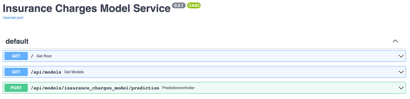
As you can see the Insurance Charges Model got it's own endpoint.
We can try out the service with this command:
!curl -X 'POST' \
  'http://127.0.0.1:8000/api/models/insurance_charges_model/prediction' \
  -H 'accept: application/json' \
  -H 'Content-Type: application/json' \
  -d "{ \
        \"age\": 42, \
        \"sex\": \"female\", \
        \"bmi\": 24.0, \
        \"children\": 2, \
        \"smoker\": false, \
        \"region\": \"northwest\" \
    }"
{"charges":8640.78}
By accessing the model's endpoint we were able to make a prediction. We got exactly the same prediction as when we installed the model in the example above.
By using the MLModel base class provided by the ml_base package and the REST service framework provided by the rest_model_service package we're able to quickly stand up a service to host the model.
Creating a Load Testing Script
To create a load testing script, we'll use the locust package. We'll install the package with this command:
!pip install locust

clear_output()
In order to run a load test with locust, we need to define what requests the locust package will make to the model service. To do this we need to define an HttpUser class.
from locust import HttpUser, constant_throughput, task
from faker import Faker


class ModelServiceUser(HttpUser):
    wait_time = constant_throughput(1)

    @task
    def post_prediction(self):
        faker = Faker()

        record = {
            "age": faker.random_int(min=18, max=65),
            "sex": faker.random_choices(elements=("male", "female"), length=1)[0],
            "bmi": faker.random_int(min=15000, max=50000) / 1000.0,
            "children": faker.random_int(min=0, max=5),
            "smoker": faker.boolean(),
            "region": faker.random_choices(
                elements=("southwest", "southeast", "northwest", "northeast"), length=1)[0]
        }
        self.client.post("/api/models/insurance_charges_model/prediction", json=record)
The class above makes a single request to the prediction endpoint in the model service, generating a random sample using the same code that we used to profile the model above. The load test consists of a single task that will be executed over and over, but we can easily add other tasks if we wanted to use the model in different ways. The wait_time attribute of the class is set to a constant throughout of 1, which means that each task will be executed at most 1 time per second by each simulated user in the load test. We can use this throuput and the number of concurrent users to create a realistic load test profile.
The code above is saved in the load_test.py file in the tests folder in the repository. We can launch a load test with this command:
locust -f tests/load_test.py
The load test process starts up a web app that can be accessed locally on http://127.0.0.1:8089.
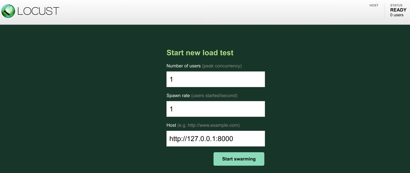
To start a load test, the locust web app asks for the number of users to simulate, the spawn rate of users, and the base url of the service to send requests to. We set the number of users to 1, the spawn rate to 1 per second, and the url to the service instance that is currently running on the local host.
When we click on the "Start swarming" button, the load test starts and we can see this screen:
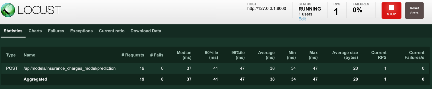
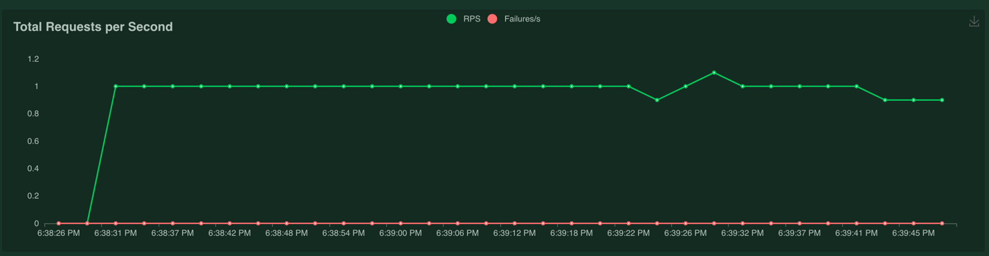
The load test is running and sending requests to the model service at the rate of one request per second from one user. The web UI also shows some charts in a separate tab in the UI, for example the total requests per second:
The response time is milliseconds:
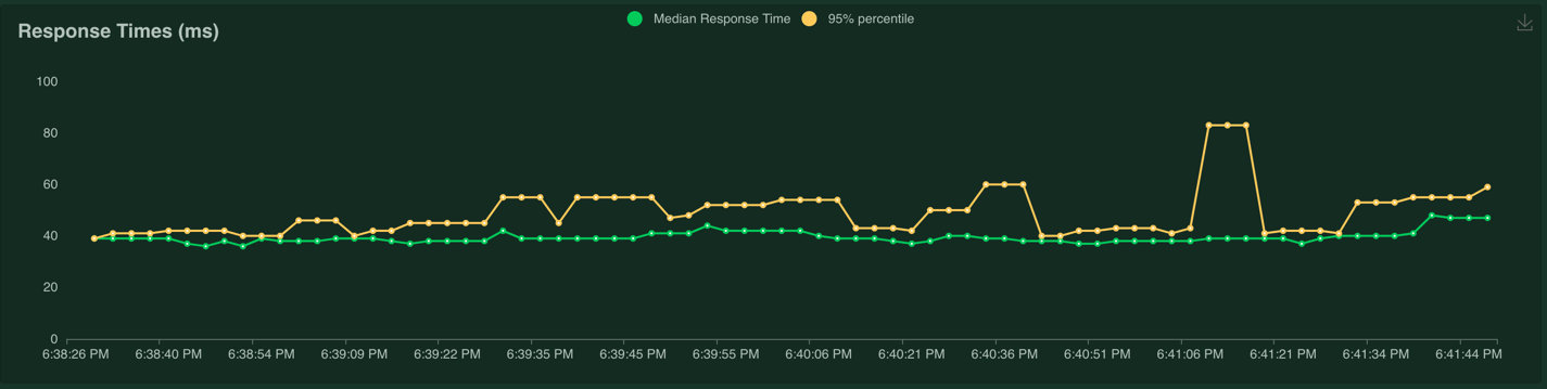
And the number of users:
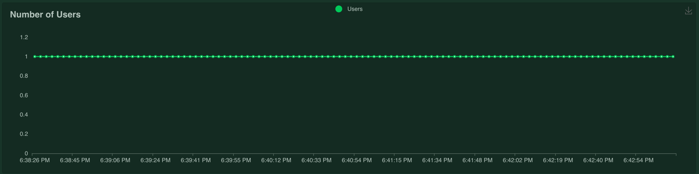
When we're ready to stop the load test, we can click on the "Stop" button in the upper right corner.
Determining whether the model service meets the SLO is as simple as inspecting the "Statistics" tab.
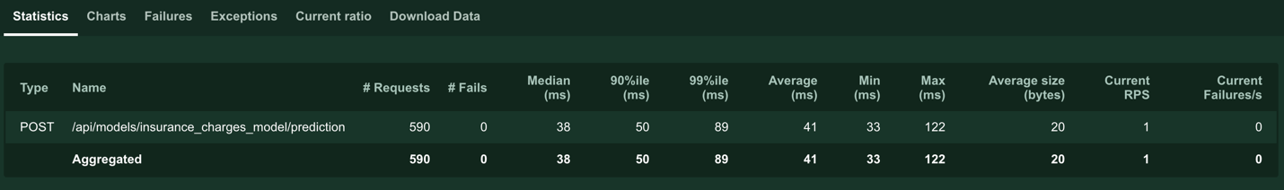
We can see that the maximum latency of the prediction request was 122 milliseconds, which does not meet our SLO of 100 ms. However, using the max is often a noisy measurement because it can be affected by many different environmental factors. It's better to use the 90th or 99th percentile. In this case the 99th percentile is 89 ms, which does meet our SLO.
This load test is not very realistic because it only has one concurrent user. In the next load tests, we'll add more concurrent users to make it more realistic.
Adding Shape to the Load Test
Right now the load test script is able to simulate one concurrent user making one request to the service per second. This is a good place to start, but we should test the service with more users. The load test is also designed to run indefinitely with the same number of users. We will add "shape" to the load test by raising the number of users over of time and then lowering the number of users back down. This will show us the performance of the service over many load conditions. We'll also stop the load test after the load test returns to the baseline, this will help us to automate the load test later.
To add a "shape" to the load test, we'll add a class that is a subclass of LoadTestShape to the load test file:
from locust import LoadTestShape


class StagesShape(LoadTestShape):
    """Simple load test shape class."""

    stages = [
        {"duration": 30, "users": 1, "spawn_rate": 1},
        {"duration": 60, "users": 2, "spawn_rate": 1},
        {"duration": 90, "users": 3, "spawn_rate": 1},
        {"duration": 120, "users": 4, "spawn_rate": 1},
        {"duration": 150, "users": 5, "spawn_rate": 1},
        {"duration": 180, "users": 4, "spawn_rate": 1},
        {"duration": 210, "users": 3, "spawn_rate": 1},
        {"duration": 240, "users": 2, "spawn_rate": 1},
        {"duration": 270, "users": 1, "spawn_rate": 1}
    ]

    def tick(self):
        run_time = self.get_run_time()

        for stage in self.stages:
            if run_time < stage["duration"]:
                tick_data = (stage["users"], stage["spawn_rate"])
                return tick_data
        # returning None to stop the load test
        return None
The tick() method is called once per second by the locust framework to determine the number of users needed and how fast to spawn the users. The tick() method looks up the desired number of users and spawn rate from the stages list. The tick() method simply iterates through the list until it finds the correct stage to use based on the number of elapsed seconds since the beginning of the load test. We defined 9 stages in the stages list, with each stage taking 30 seconds, the max number of concurrent users will be 5.
To run the load test, simply execute the same command as above:
locust -f tests/load_test.py
The load test will start when we press the "Start swarming" button, as before. However, this load test will vary the number of users according to the shape defined in the class. Since the number of users and spawn rate is determined by the shape class, we dont need to provide these to start the load test.
The load test runs for six minutes and the number of users chart looks like this:
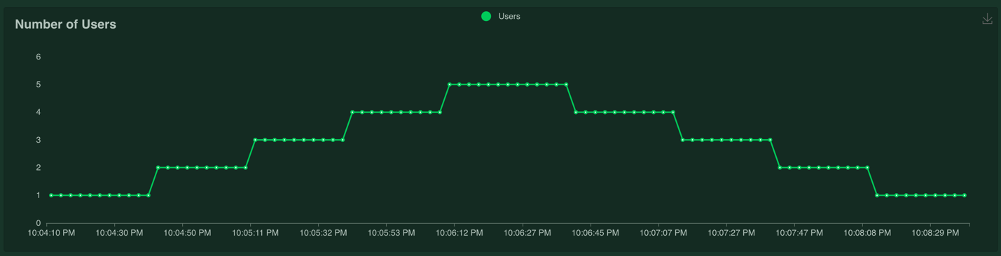
The response time chart looks like this:
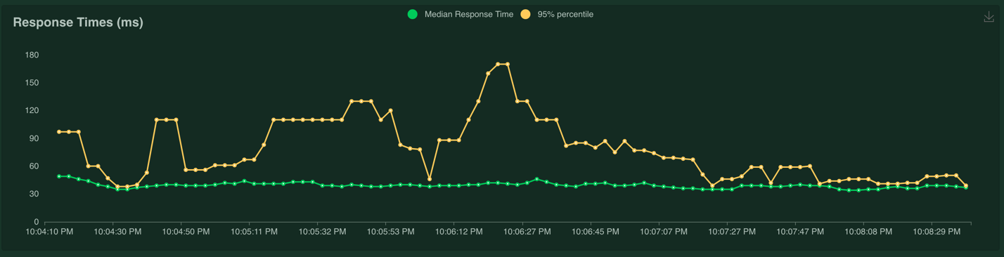
The response time of the service definitely suffered when the number of users went above 1, and the maximum response time of the service was 225 ms. It looks like a single instance of the model service cannot handle much more than 1 concurrent users making one request per second.
The requests per second chart looks like this:
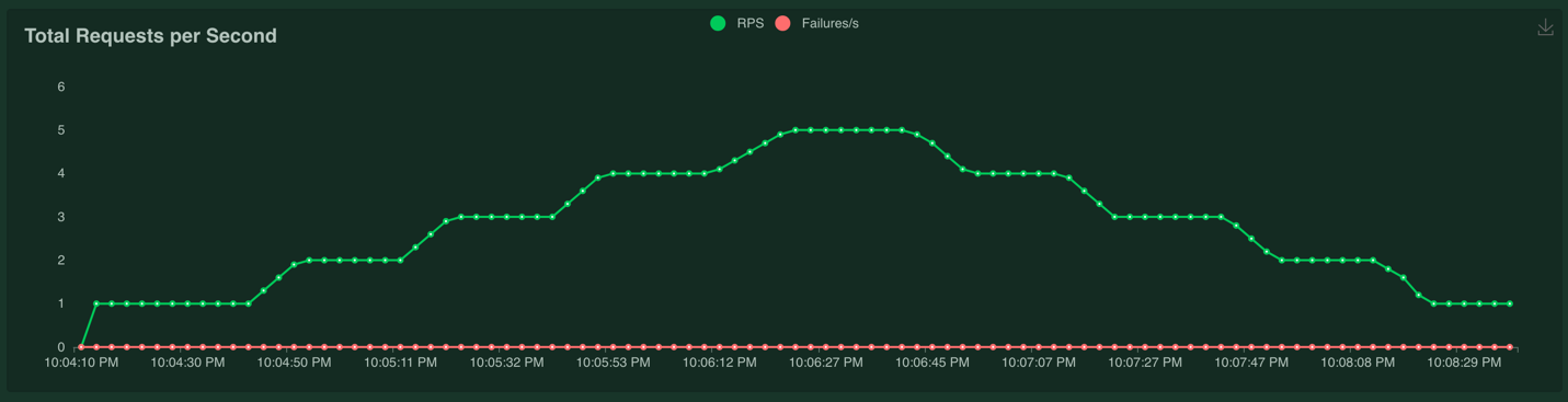
The number of requests per second scaled with the number of users because we're making one request per second per user.
Adding Service Level Objectives
Right now, the load test script simply runs the load test and displays the results on a webpage. However, we can make it more useful by adding support for SLOs. For example, we can have the load test fail if the latency of any request is above a certain threshold, or if the average latency of all requests is above a certain threshold.
We'll add support for checking the following SLOs: - latency, we'll check that the latency at the 99th percentile is less than 100 ms - error rate, we'll check that there are no errors returned on any request - throughput, we'll check that the service can handle at least 5 requests per second
To do this we'll add a listener function that receives events from the locust package:
import logging

logger = logging.getLogger(__name__)


@events.test_stop.add_listener
def on_test_stop(environment, **kwargs):
    process_exit_code = 0

    max_requests_per_second = max(
        [requests_per_second for requests_per_second in environment.stats.total.num_reqs_per_sec.values()])

    if environment.stats.total.fail_ratio > 0.0:
        logger.error("Test failed because there was one or more errors.")
        process_exit_code = 1

    if environment.stats.total.get_response_time_percentile(0.99) > 100:
        logger.error("Test failed because the response time at the 99th percentile was above 100 ms. The 99th "
                     "percentile latency is '{}'.".format(environment.stats.total.get_response_time_percentile(0.99)))
        process_exit_code = 1

    if max_requests_per_second < 5:
        logger.error(
            "Test failed because the max requests per second never reached 5. The max requests per second "
            "is: '{}'.".format(max_requests_per_second))
        process_exit_code = 1

    environment.process_exit_code = process_exit_code
The on_test_quitting function is going to execute at the end of every load test. This function can access all of the statistics saved by the load test, we can check the different conditions by accessing the statistics. If any of the SLOs are not met, we set the process exit code to be 1, which signals a failure to the operating system.
To run the load test, execute the same command as above. When the load test finishes, the process will output the results to the command line. In this case the load test failed with this output:
Test failed because the response time at the 99th percentile was above 100 ms. The 99th percentile latency is '180.0'.
Running a Headless Load Test
The locust package can also run load test without the web UI. This is useful for doing automated load tests that run in a server, without anyone watching the UI. The command is:
locust -f tests/load_test.py --host=http://127.0.0.1:8000 --headless --loglevel ERROR --csv=./load_test_report/load_test --html ./load_test_report/load_test_report.html
Once the test finishes, we see the same error as above because the load test did not meet the SLO required. The error message is:
Test failed because the response time at the 99th percentile was above 100 ms. The 99th percentile latency is '180.0'.
All of the code for the load test script is found in the "test/load_test.py" file in the repository for this blog post. The results are stored in CSV files and an HTML file in the "load_test_report" folder.
Building a Docker Image
Now that we have a working model and model service, we'll need to deploy it somewhere. We'll start by deploying the service locally using Docker.
Let's create a docker image and run it locally. The docker image is generated using instructions in the Dockerfile:
# syntax=docker/dockerfile:1
FROM python:3.9-slim

ARG BUILD_DATE

LABEL org.opencontainers.image.title="Load Tests for ML Models"
LABEL org.opencontainers.image.description="Load tests for machine learning models."
LABEL org.opencontainers.image.created=$BUILD_DATE
LABEL org.opencontainers.image.authors="6666331+schmidtbri@users.noreply.github.com"
LABEL org.opencontainers.image.source="https://github.com/schmidtbri/load-tests-for-ml-models"
LABEL org.opencontainers.image.version="0.1.0"
LABEL org.opencontainers.image.licenses="MIT License"
LABEL org.opencontainers.image.base.name="python:3.9-slim"

WORKDIR /service

ARG USERNAME=service-user
ARG USER_UID=1000
ARG USER_GID=1000

RUN apt-get update

# create a user
RUN groupadd --gid $USER_GID $USERNAME \
    && useradd --uid $USER_UID --gid $USER_GID -m $USERNAME \
    && apt-get install --assume-yes --no-install-recommends sudo \
    && echo $USERNAME ALL=\(root\) NOPASSWD:ALL > /etc/sudoers.d/$USERNAME \
    && chmod 0440 /etc/sudoers.d/$USERNAME

# installing git because we need to install the model package from it's own github repository
RUN apt-get install --assume-yes --no-install-recommends git

RUN apt-get clean \
    && rm -rf /var/lib/apt/lists/*

# installing dependencies first in order to speed up build by using cached layers
COPY ./service_requirements.txt ./service_requirements.txt
RUN pip install -r service_requirements.txt

COPY ./configuration ./configuration
COPY ./LICENSE ./LICENSE

CMD ["uvicorn", "rest_model_service.main:app", "--host", "0.0.0.0", "--port", "8000"]

USER $USERNAME
The Dockerfile is used by this docker command to create a docker image:
!docker build -t insurance_charges_model_service:latest ../

clear_output()
To make sure everything worked as expected, we'll look through the docker images in our system:
!docker image ls | grep insurance_charges_model_service
insurance_charges_model_service latest 446f5f06805f 37 seconds ago 1.25GB
Next, we'll start the image to see if everything is working as expected.
!docker run -d \
    -p 8000:8000 \
    -e REST_CONFIG=./configuration/local_rest_config.yaml \
    --name insurance_charges_model_service \
    insurance_charges_model_service:latest
44c4794160f941e44d1670b70c7fd5722c41bf0c2e470a0b0c8648c966b9923b
The service should be accessible on port 8000 of localhost, so we'll try to make a prediction:
!curl -X 'POST' \
  'http://127.0.0.1:8000/api/models/insurance_charges_model/prediction' \
  -H 'accept: application/json' \
  -H 'Content-Type: application/json' \
  -d "{ \
        \"age\": 42, \
        \"sex\": \"female\", \
        \"bmi\": 24.0, \
        \"children\": 2, \
        \"smoker\": false, \
        \"region\": \"northwest\" \
    }"
{"charges":8640.78}
We'll use the model service Docker image to deploy the model service and automate the load test later.
Now that we're done with the local redis instance we'll stop and remove the docker container.
!docker kill insurance_charges_model_service
!docker rm insurance_charges_model_service
insurance_charges_model_service
insurance_charges_model_service
Deploying the Model Service
To show the system in action, we’ll deploy the service and the Redis instance to a Kubernetes cluster. A local cluster can be easily started by using minikube. Installation instructions can be found here.
To start the minikube cluster execute this command:
!minikube start
😄 minikube v1.26.1 on Darwin 12.5
✨ Using the virtualbox driver based on existing profile
👍 Starting control plane node minikube in cluster minikube
🔄 Restarting existing virtualbox VM for "minikube" ...
🐳 Preparing Kubernetes v1.24.3 on Docker 20.10.17 ...[K[K[K[K
▪ controller-manager.horizontal-pod-autoscaler-sync-period=5s
🔎 Verifying Kubernetes components...
▪ Using image k8s.gcr.io/metrics-server/metrics-server:v0.6.1
▪ Using image gcr.io/k8s-minikube/storage-provisioner:v5
▪ Using image kubernetesui/dashboard:v2.6.0
▪ Using image kubernetesui/metrics-scraper:v1.0.8
🌟 Enabled addons: dashboard
🏄 Done! kubectl is now configured to use "minikube" cluster and "default" namespace by default
We'll need to use the Kubernetes Dashboard to view details about the model service. We can start it up in the minikube cluster with this command:
minikube dashboard --url
The command starts up a proxy that must keep running in order to forward the traffic to the dashboard UI in the minikube cluster.
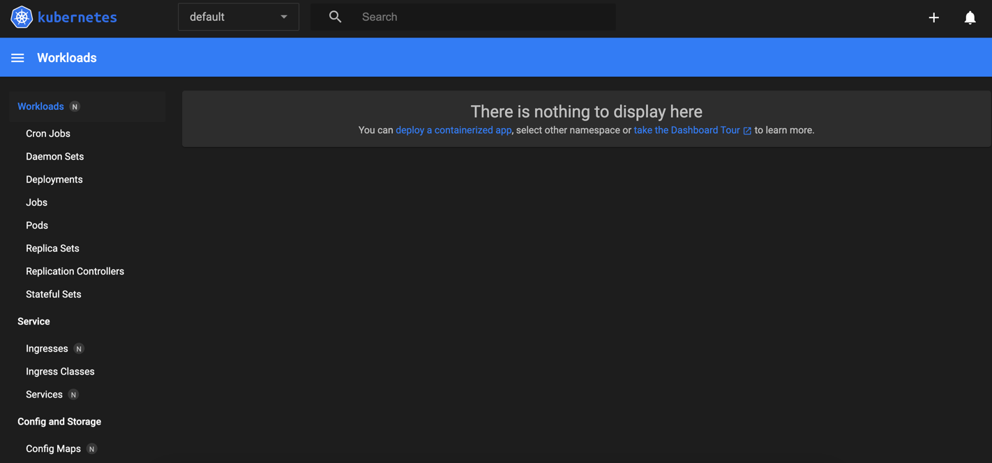
The dashboard UI looks like this:
We'll also need to use the metrics server in Kubernetes. We can enable that in minikube with this command:
!minikube addons enable metrics-server
💡  metrics-server is an addon maintained by Kubernetes. For any concerns contact minikube on GitHub.
You can view the list of minikube maintainers at: https://github.com/kubernetes/minikube/blob/master/OWNERS
    ▪ Using image k8s.gcr.io/metrics-server/metrics-server:v0.6.1
🌟  The 'metrics-server' addon is enabled
Let's view all of the pods running in the minikube cluster to make sure we can connect.
!kubectl get pods -A
NAMESPACE              NAME                                         READY   STATUS    RESTARTS       AGE
kube-system            coredns-6d4b75cb6d-wrrwr                     1/1     Running   16 (22h ago)   23d
kube-system            etcd-minikube                                1/1     Running   16 (22h ago)   23d
kube-system            kube-apiserver-minikube                      1/1     Running   16 (22h ago)   23d
kube-system            kube-controller-manager-minikube             1/1     Running   2 (22h ago)    24h
kube-system            kube-proxy-5n4t9                             1/1     Running   15 (22h ago)   23d
kube-system            kube-scheduler-minikube                      1/1     Running   14 (22h ago)   23d
kube-system            metrics-server-8595bd7d4c-ptcsp              1/1     Running   12 (22h ago)   4d2h
kube-system            storage-provisioner                          1/1     Running   25 (24s ago)   23d
kubernetes-dashboard   dashboard-metrics-scraper-78dbd9dbf5-xslpl   1/1     Running   8 (22h ago)    4d2h
kubernetes-dashboard   kubernetes-dashboard-5fd5574d9f-vbtnd        1/1     Running   10 (22h ago)   4d2h
The pods running the kubernetes dashboard and metrics server appear in the kube-system and kubernetes-dashboard namespaces.
Creating a Kubernetes Namespace
Now that we have a cluster and are connected to it, we'll create a namespace to hold the resources for our model deployment. The resource definition is in the kubernetes/namespace.yaml file. To apply the manifest to the cluster, execute this command:
!kubectl create -f ../kubernetes/namespace.yaml
namespace/model-services created
To take a look at the namespaces, execute this command:
!kubectl get namespace
NAME                   STATUS   AGE
default                Active   23d
kube-node-lease        Active   23d
kube-public            Active   23d
kube-system            Active   23d
kubernetes-dashboard   Active   4d2h
model-services         Active   1s
The new namespace appears in the listing along with other namespaces created by default by the system. To use the new namespace for the rest of the operations, execute this command:
!kubectl config set-context --current --namespace=model-services
Context "minikube" modified.
Creating a Model Deployment and Service
The model service is deployed by using Kubernetes resources. These are:
- ConfigMap: a set of configuration options, in this case it is a simple YAML file that will be loaded into the running container as a volume mount. This resource allows us to change the configuration of the model service without having to modify the Docker image.
- Deployment: a declarative way to manage a set of pods, the model service pods are managed through the Deployment.
- Service: a way to expose a set of pods in a Deployment, the model services is made available to the outside world through the Service, the service type is LoadBalancer which means that a load balancer will be created for the service.
These resources are defined in the ./kubernetes/model_service.yaml file in the project repository.
To start the model service, first we'll need to send the docker image from the local docker daemon to the minikube image cache:
!minikube image load insurance_charges_model_service:latest
We can view the images in the minikube cache like this:
!minikube cache list
insurance_charges_model_service:latest
The model service resources are created within the Kubernetes cluster with this command:
!kubectl apply -f ../kubernetes/model_service.yaml
configmap/model-service-configuration created
deployment.apps/insurance-charges-model-deployment created
service/insurance-charges-model-service created
Let's get the names of the pods that are running the service:
!kubectl get pods
NAME                                                  READY   STATUS    RESTARTS   AGE
insurance-charges-model-deployment-5454fc7cfb-rhl2t   1/1     Running   0          4s
To make sure the service started up correctly, we'll check the logs of the single pod running the service:
!kubectl logs insurance-charges-model-deployment-5454fc7cfb-rhl2t
/usr/local/lib/python3.9/site-packages/tpot/builtins/__init__.py:36: UserWarning: Warning: optional dependency `torch` is not available. - skipping import of NN models.
  warnings.warn("Warning: optional dependency `torch` is not available. - skipping import of NN models.")
INFO:     Started server process [1]
INFO:     Waiting for application startup.
INFO:     Application startup complete.
INFO:     Uvicorn running on http://0.0.0.0:8000 (Press CTRL+C to quit)
Looks like the server process started correctly in the Docker container. The UserWarning is generated when we instantiate the model object, which means everything is running as expected.
The deployment and service for the model service were created together. You can see the new service with this command:
!kubectl get services
NAME                              TYPE       CLUSTER-IP      EXTERNAL-IP   PORT(S)        AGE
insurance-charges-model-service   NodePort   10.98.168.223   <none>        80:31687/TCP   48s
Minikube exposes the service on a local port, we can get a link to the endpoint with this command:
minikube service insurance-charges-model-service --url -n model-services
The command output this URL:
http://192.168.59.100:31687
The command must keep running to keep the tunnel open to the running model service in the minikube cluster.
To make a prediction, we'll hit the service with a request:
!curl -X 'POST' \
  'http://192.168.59.100:31687/api/models/insurance_charges_model/prediction' \
  -H 'accept: application/json' \
  -H 'Content-Type: application/json' \
  -d "{ \
        \"age\": 65, \
        \"sex\": \"male\", \
        \"bmi\": 22, \
        \"children\": 5, \
        \"smoker\": true, \
        \"region\": \"southwest\" \
    }"
{"charges":25390.95}
We have the model service up and running in the local minikube cluster!
Running the Load Test
We can run the load test by using the IP address and port of the service running in minikube.
locust -f tests/load_test.py --host=http://192.168.59.100:31687 --headless --loglevel ERROR --csv=./load_test_report/load_test --html ./load_test_report/load_test_report.html
While the load test is running, we'll check the CPU usage of the single pod running the model service every 15 seconds:
%%bash

kubectl top pods

while sleep 15; do
    kubectl top pods | grep insurance-charges-model-deployment
done
NAME                                                  CPU(cores)   MEMORY(bytes)
insurance-charges-model-deployment-5454fc7cfb-rhl2t   4m           104Mi
insurance-charges-model-deployment-5454fc7cfb-rhl2t   27m          104Mi
insurance-charges-model-deployment-5454fc7cfb-rhl2t   27m          104Mi
insurance-charges-model-deployment-5454fc7cfb-rhl2t   27m          104Mi
insurance-charges-model-deployment-5454fc7cfb-rhl2t   27m          104Mi
insurance-charges-model-deployment-5454fc7cfb-rhl2t   132m         105Mi
insurance-charges-model-deployment-5454fc7cfb-rhl2t   132m         105Mi
insurance-charges-model-deployment-5454fc7cfb-rhl2t   132m         105Mi
insurance-charges-model-deployment-5454fc7cfb-rhl2t   132m         105Mi
insurance-charges-model-deployment-5454fc7cfb-rhl2t   198m         107Mi
insurance-charges-model-deployment-5454fc7cfb-rhl2t   198m         107Mi
insurance-charges-model-deployment-5454fc7cfb-rhl2t   198m         107Mi
insurance-charges-model-deployment-5454fc7cfb-rhl2t   198m         107Mi
insurance-charges-model-deployment-5454fc7cfb-rhl2t   200m         107Mi
insurance-charges-model-deployment-5454fc7cfb-rhl2t   200m         107Mi
insurance-charges-model-deployment-5454fc7cfb-rhl2t   200m         107Mi
insurance-charges-model-deployment-5454fc7cfb-rhl2t   200m         107Mi
insurance-charges-model-deployment-5454fc7cfb-rhl2t   94m          107Mi
insurance-charges-model-deployment-5454fc7cfb-rhl2t   94m          107Mi
insurance-charges-model-deployment-5454fc7cfb-rhl2t   94m          107Mi
Process is interrupted.
We can clearly see how the CPU usage is affected as the load goes from 1 user to 5 users. The CPU request for the deployment is 100 millicores, and the CPU usage goes as high as 200 millicores. The memory usage did not change very much based on the load.
The load test output this error message right before stopping:
Test failed because the response time at the 99th percentile was above 100 ms. The 99th percentile latency is '3300.0'.
We can see that the single instance of the service running in Kubernetes is not enough to meet the requirements of the load test, and that the CPU usage is the limiting factor.
Adding Autoscaling to the Model Service
Kubernetes supports autoscaling, which is the ability to change the resources assigned to a service based on the current load on the service. We'll be doing horizontal scaling, which means that the number of replicas increases and decreases according to the load. Kubernetes supports this kind of autoscaling through the HorizontalAutoScaler resource.
The HorizontalAutoScaler resource is defined like this:
apiVersion: autoscaling/v2
kind: HorizontalPodAutoscaler
metadata:
  name: insurance-charges-model-autoscaler
spec:
  scaleTargetRef:
    apiVersion: apps/v1
    kind: Deployment
    name: insurance-charges-model-deployment
  minReplicas: 1
  maxReplicas: 10
  metrics:
  - type: Resource
    resource:
      name: cpu
      target:
        type: Utilization
        averageUtilization: 50
This resource is defined in the /kubernetes/autoscaler.yaml file in the repository.
The HorizontalPodAutoscaler resource simply states that each pod of the deployment be kept at 50% CPU utilization. Since the pods of our service request 100 millicores, the autoscaler controller will step in whenever the CPU usage goes above 50 millicores and add a replica to the deployment.
We can deploy the HorizontalPodAutoscaler resource with this command:
!kubectl apply -f ../kubernetes/autoscaler.yaml
horizontalpodautoscaler.autoscaling/insurance-charges-model-autoscaler created
We can view the number of replicas in the Deployment in the Kubernetes Dashboard:
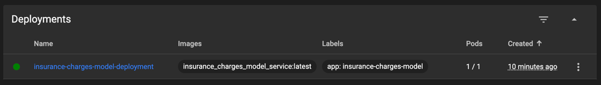
The deployment currently has 1 pod, with 1 requested pod.
We can also see the HorizontalPodAutoscaler:

The number of replicas is currently set to 1, the autoscaler will increase and decrease this number automatically.
Let's try running the load test with more concurrent users and see if we can trigger an autoscaling event.
locust -f tests/load_test.py --host=http://192.168.59.100:31687 --headless --loglevel ERROR --csv=./load_test_report/load_test --html ./load_test_report/load_test_report.html
While it's running, let's watch the deployment for the number of replicas:
%%bash

kubectl get deployment insurance-charges-model-deployment

while sleep 15; do
    kubectl get deployment insurance-charges-model-deployment | grep insurance-charges-model-deployment
done
NAME                                 READY   UP-TO-DATE   AVAILABLE   AGE
insurance-charges-model-deployment   1/1     1            1           14m
insurance-charges-model-deployment   1/1     1            1           14m
insurance-charges-model-deployment   1/1     1            1           15m
insurance-charges-model-deployment   2/2     2            2           15m
insurance-charges-model-deployment   2/2     2            2           15m
insurance-charges-model-deployment   2/2     2            2           15m
insurance-charges-model-deployment   2/2     2            2           16m
insurance-charges-model-deployment   4/4     4            4           16m
insurance-charges-model-deployment   4/4     4            4           16m
insurance-charges-model-deployment   4/4     4            4           16m
insurance-charges-model-deployment   4/4     4            4           17m
insurance-charges-model-deployment   6/6     6            6           17m
insurance-charges-model-deployment   6/6     6            6           17m
insurance-charges-model-deployment   6/6     6            6           17m
insurance-charges-model-deployment   6/6     6            6           18m
insurance-charges-model-deployment   6/6     6            6           18m
insurance-charges-model-deployment   6/6     6            6           18m
insurance-charges-model-deployment   6/6     6            6           18m
insurance-charges-model-deployment   6/6     6            6           19m
insurance-charges-model-deployment   6/6     6            6           19m
insurance-charges-model-deployment   6/6     6            6           19m
insurance-charges-model-deployment   6/6     6            6           19m
insurance-charges-model-deployment   6/6     6            6           20m
insurance-charges-model-deployment   6/6     6            6           20m
insurance-charges-model-deployment   6/6     6            6           20m
insurance-charges-model-deployment   6/6     6            6           20m
insurance-charges-model-deployment   6/6     6            6           21m
insurance-charges-model-deployment   6/6     6            6           21m
Process is interrupted.
The increasing caused the number of replicas to go up to 6.
Autoscaling can be triggered by using other metrics, such as memory usage. Autoscaling can ensure that a service can scale to meet the current needs of the clients of the system.
Deleting the Resources
Now that we're done with the service we need to destroy the resources.
To delete the service autoscaler, execute this command:
!kubectl delete -f ../kubernetes/autoscaler.yaml
horizontalpodautoscaler.autoscaling "insurance-charges-model-autoscaler" deleted
To delete the model service, we'll execute this command:
!kubectl delete -f ../kubernetes/model_service.yaml
configmap "model-service-configuration" deleted
deployment.apps "insurance-charges-model-deployment" deleted
service "insurance-charges-model-service" deleted
To delete the namespace:
!kubectl delete -f ../kubernetes/namespace.yaml
namespace "model-services" deleted
Lastly, to stop the kubernetes cluster, execute these commands:
!minikube stop
✋  Stopping node "minikube"  ...
🛑  1 node stopped.
Closing
In this blog post we showed how to create a load testing script for a machine learning model that is deployed within a RESTful service. The load testing script is able to generate random inputs for the model. We also showed how to add a shape to the load test in order to simplify load testing and how to add SLOs to the load testing script so that we can quickly tell if the model and model service are able to meet the requirements of the deployment. Lastly, we deployed the model service to a Kubernetes and showed how to implement autoscaling so that the model service can meet the SLO adaptively.