Property-Based Testing for ML Models
Introduction
Property-based testing is a form of software testing that allows developers to write more comprehensive tests for software components. Property-based tests work by asserting that certain properties of the software component under test hold over a wide range of inputs.
Property-based tests rely on the generation of inputs for a component and are a form of generative testing. When doing property-based testing it is useful to think in terms of invariants within the software component that we are testing. An invariant is a condition or assumption that we expect will never be violated by the component.
Generative software testing is a type of testing in which a developer does not have to come up with test cases manually. To accomplish this, an engine is used that can come up with any number of test cases, as long as we're able to state our requirements for the test cases clearly and concisely. When the engine generates a test case for us, we send it to the code that we are testing and see if any errors come up. Generative testing is a form of black box testing because we don't really know much about the internals of the component that is under test, we just know how to structure its input in the correct way. Once a test case is generated, we test by making sure that the component returns valid output or that it is not in an invalid state.
Machine learning models are just like any other software component, they require input and provide an output. In fact, ML models are some of the simplest software components that make up a software system because they usually only have one function: the "predict" function. The prediction usually only requires one object, and the prediction result is also a single object. Because of these factors, ML models are actually great candidates for property-based testing. In this blog post, we'll focus on testing the input and output schemas of the model and we'll make sure that the model is able to accept the inputs that it says that it can accept. In terms of invariants, we'll be testing that the model can handle any input that is within its stated input schema.
In this blog post, we'll do property-based testing of an ML model and a RESTful model service that we'll build around the same model. To do property-based testing we'll use the hypothesis package, and to do property-based testing on the model service we'll use the schemathesis package.
Package Structure
-   mobile_handset_price_model
    -   model_files (output files from model training)
    -   prediction (package for the prediction code)
        -   __init__.py
        -   model.py (prediction code)
        -   schemas.py (model input and output schemas)
        -   transformers.py (data transformers)
    -   training (package for the training code)
        -   data_exploration.ipynb (data exploration code)
        -   data_preparation.ipynb (data preparation code)
        -   model_training.ipynb (model training code)
        -   model_validation.ipynb (model validation code)
    -   tests (unit tests for model codel)
    -   Makefile
    -   requirements.txt (list of dependencies)
    -   rest_config.yaml (configuration for REST model service)
    -   service_contract.yaml (OpenAPI service contract)
    -   setup.py
    -   test_requirements.txt (test dependencies)
All of the code is available in a github repository.
Creating a Model
To be able to do property-based testing on an ML model, we'll need to have a model to work with. In this section we will get a dataset, explore it, preprocess it, train a model on it, and validate the resulting model.
Getting Data
In order to train a model, we first need to have a dataset. We went into Kaggle and found a dataset that contains mobile handset price information. To make it easy to download the dataset, we installed the kaggle python package and then we executed these commands to download the data and unzip it into the data folder in the project:
mkdir -p data
kaggle datasets download -d iabhishekofficial/mobile-price-classification/tasks -p ./data --unzip
To make it even easier to download the data, we added a Makefile target for the commands:
download-dataset:
    mkdir -p data
    kaggle datasets download -d iabhishekofficial/mobile-price-classification/tasks -p ./data --unzip
Now all we need to do to get the data is execute this command:
make download-data
Instead of having to remember how to get the data needed to do modeling, I always try to create a repeatable and documented process for creating the dataset. We also need to make sure to never store the dataset in source control, so we\'ll add this line to the .gitignore file:
data/
Training a Model
Data Exploration
In order to create a model, we'll first explore the data. Before we can do that, we need to first load the data and do some basic housekeeping.
data = pd.read_csv("../../data/train.csv")
The datatypes of the columns are:
data.dtypes
battery_power int64
blue          int64
clock_speed   float64
dual_sim      int64
fc            int64
four_g        int64
int_memory    int64
m_dep         float64
mobile_wt     int64
n_cores       int64
pc            int64
px_height     int64
px_width      int64
ram           int64
sc_h          int64
sc_w          int64
talk_time     int64
three_g       int64
touch_screen  int64
wifi          int64
price_range   int64
dtype: object
In order to more easily work with the data, we\'ll rename some of the columns so that they have clearer names:
columns = {
    "blue": "has_bluetooth",
    "dual_sim": "has_dual_sim",
    "fc": "front_camera_megapixels",
    "four_g": "has_four_g",
    "int_memory": "internal_memory",
    "m_dep": "depth",
    "mobile_wt": "weight",
    "n_cores": "number_of_cores",
    "pc": "primary_camera_megapixels",
    "px_height": "pixel_resolution_height",
    "px_width": "pixel_resolution_width",
    "sc_h": "screen_height",
    "sc_w": "screen_width",
    "three_g": "has_three_g",
    "touch_screen": "has_touch_screen",
    "wifi": "has_wifi"
}

data = data.rename(columns=columns)
We also need to get the unique values of the variable we intend to use as the target variable:
data["price_range"].unique()
array([1, 2, 3, 0])
The target variable holds categorical values.
To finish the data exploration we'll use the pandas_profiling package. This package is able to take a pandas dataframe and quickly create a full report about the dataset in the dataframe. Here are some simple statistics found by pandas_profiling:
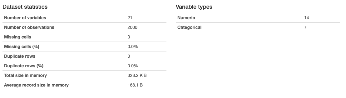
The dataset has 21 variables in total, with 14 numeric variables and 7 categorical variables. There are 2000 samples, with no missing values or duplicate values. After examining the report, we can see that the categorical variables all hold only two values, for example the "has_bluetooth" variable:
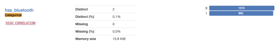
From this we can see that these are really just boolean values, we'll use this later in order to simplify the input schema of the model.
The data exploration is in this notebook.
Preparing the Data
To prepare the data for modeling, we'll first create lists of categorical, numerical, and boolean variables:
categorical_cols = []

numerical_columns = [
    "battery_power",
    "clock_speed",
    "front_camera_megapixels",
    "internal_memory",
    "depth",
    "weight",
    "number_of_cores",
    "primary_camera_megapixels",
    "pixel_resolution_height",
    "pixel_resolution_width",
    "ram",
    "screen_height",
    "screen_width",
    "talk_time"
]

boolean_columns = [
    "has_bluetooth",
    "has_dual_sim",
    "has_four_g",
    "has_three_g",
    "has_touch_screen",
    "has_wifi",
]
Because all of the categorical variables are in fact boolean variables, we don\'t have any variables in the "categorical_cols" list. Next, we'll create a transformer that will work with the numerical variables:
numerical_transformer = Pipeline(steps=[
    ("imputer", SimpleImputer(strategy="mean")),
    ("scaler", StandardScaler())
])
Next, we\'ll create a transformer that is able to convert the values in the boolean columns to boolean values:
boolean_transformer = BooleanTransformer(true_value=1, false_value=0)
Lastly, we'll combine both transformers using a ColumnTransformer:
column_transformer = ColumnTransformer(
    remainder="passthrough",
    transformers=[
        ("numerical", numerical_transformer, numerical_columns),
        ("boolean", boolean_transformer, boolean_columns)
    ]
)
Now we can save the transformer object so we can fit it to the data later:
joblib.dump(column_transformer, "column_transformer.joblib")
The data preparation code is in this notebook.
Training a Model
Now that we have the data transformations built, we can train a model. To do that, we'll first create lists of the predictor variables and the target column:
feature_columns = [
    "battery_power",
    "has_bluetooth",
    "clock_speed",
    "has_dual_sim",
    "front_camera_megapixels",
    "has_four_g",
    "internal_memory",
    "depth",
    "weight",
    "number_of_cores",
    "primary_camera_megapixels",
    "pixel_resolution_height",
    "pixel_resolution_width",
    "ram",
    "screen_height",
    "screen_width",
    "talk_time",
    "has_three_g",
    "has_touch_screen",
    "has_wifi"
]

target_column = "price_range"
Next, we'll split the dataset into training, validation, and test sets and then create dataframes for the predictor and target variables:
train, validate, test = np.split(data.sample(frac=1), [int(0.6*len(data)), int(0.8*len(data))])

X_train = train[feature_columns]
y_train = train[target_column]

X_validate = validate[feature_columns]
y_validate = validate[target_column]
We'll need the transformer we created earlier, so we'll load it from disk:
transformer = joblib.load("column_transformer.joblib")
Next, we'll create an XGBClassifier model:
model = XGBClassifier()
And combine it with the transformer to create a single pipeline:
pipeline = Pipeline(steps=[
    ("preprocessor", transformer),
    ("model", model)
])
Next, we'll fit the pipeline to the training set:
pipeline.fit(X_train, y_train)
Now we can try to make single prediction to make sure everything is working:
result = model.predict(X_validate.iloc[[0]])

print(result)
array([3])
However, this is not the real model we want, we'll do hyperparameter tuning using the hyperopt package. The hyperparameter space is defined like this:
space = {
"max_depth": hp.quniform("max_depth", 3, 18, 1),
"gamma": hp.uniform ("gamma", 1, 9),
"reg_alpha" : hp.quniform("reg_alpha", 40,180,1),
"reg_lambda" : hp.uniform("reg_lambda", 0, 1),
"colsample_bytree" : hp.uniform("colsample_bytree", 0.5, 1),
"min_child_weight" : hp.quniform("min_child_weight", 0, 10, 1),
"n_estimators": 180,
"seed": 0
}
And the objective function looks like this:
def objective(space):
    classifier = XGBClassifier(
        n_estimators=space["n_estimators"],
        max_depth=int(space["max_depth"]),
        gamma=space["gamma"],
        reg_alpha=int(space["reg_alpha"]),
        min_child_weight=int(space["min_child_weight"]),
        colsample_bytree=int(space["colsample_bytree"])
    )

    evaluation = [(X_train, y_train), (X_validate, y_validate)]
    classifier.fit(X_train, y_train, eval_set=evaluation, eval_metric="merror", early_stopping_rounds=10, verbose=False)

    predictions = classifier.predict(X_validate)
    accuracy = accuracy_score(y_validate, predictions)
    print("SCORE: ", accuracy)

    return {
    "loss": -accuracy,
    "status": STATUS_OK
    }
We'll run the hyperparameter search like this:
trials = Trials()

best_hyperparameters = fmin(fn = objective,
                            space = space,
                            algo = tpe.suggest,
                            max_evals = 100,
                            trials = trials)
The best hyperparameters found are these:
{
    'colsample_bytree': 0.7805313948569044,
    'gamma': 2.8457210780834963,
    'max_depth': 8.0,
    'min_child_weight': 8.0,
    'reg_alpha': 86.0,
    'reg_lambda': 0.23805965814363095
}
Now that we have found the best hyperparameters, we'll train the real model:
model = XGBClassifier(**best_hyperparameters)

pipeline = Pipeline(steps=[
    ("preprocessor", transformer),
    ("model", model)])

pipeline.fit(X_train, y_train)
Lastly, we can save the model object:
joblib.dump(pipeline, "model.joblib")
The model training code is in this notebook.
Validating the Model
To validate the model, we'll use the yellowbrick package. First, we\'ll load the fitted model object that was saved in a previous step:
model = joblib.load("model.joblib")
The yellowbrick package can create a classification report like this:
from yellowbrick.classifier import ClassificationReport

visualizer = ClassificationReport(model, classes=classes, support=True)
visualizer.score(X_test, y_test)
visualizer.show()
The resulting graph looks like this:
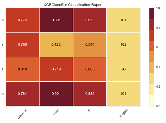
The classification report visualizer displays the precision, recall, F1, and support scores for the model for each class in the target variable.
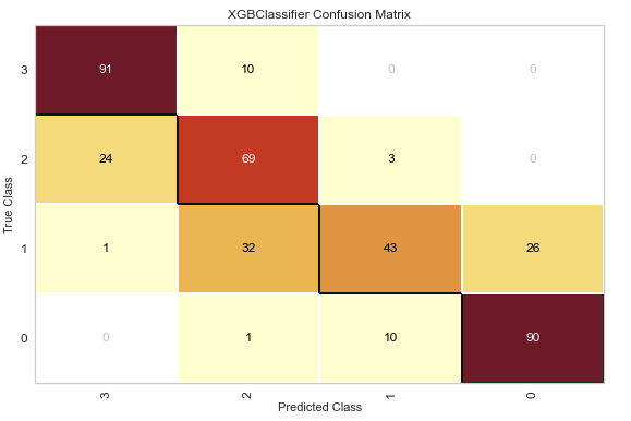
A confusion matrix is created like this:
from yellowbrick.classifier import ConfusionMatrix

visualizer = ConfusionMatrix(model, classes=classes)
visualizer.score(X_test, y_test)
visualizer.show()
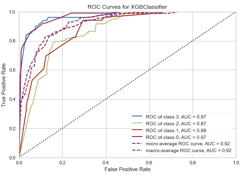
The ROC/AUC plot is created like this:
from yellowbrick.classifier import ROCAUC

visualizer = ROCAUC(model, classes=classes)
visualizer.fit(X_train, y_train)
visualizer.score(X_test, y_test)
visualizer.show()
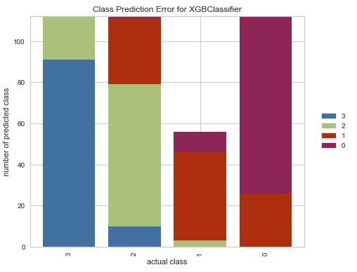
The class prediction error plot is done like this:
from yellowbrick.classifier import ClassPredictionError

visualizer = ClassPredictionError(model, classes=classes)
visualizer.score(X_test, y_test)
visualizer.show()
Now that we have a fully trained and validated model and we understand the underlying data that we used to create the model, we can move forward with writing the code that we'll use to make predictions with the model.
The model validation code is in this notebook.
Creating the Model Schemas
In order to be able to use the model, we'll need to define what it's input and output schemas are. To do this, we'll use the pydantic package to define two classes. The model input class looks like this:
class MobileHandsetPriceModelInput(BaseModel):
    """Schema for input of the model's predict method."""
    battery_power: Optional[int] = Field(None, title="battery_power", ge=500, le=2000, description="Total energy a battery can store in one time measured in mAh.")
    has_bluetooth: int = Field(..., title="has_bluetooth", description="Whether the phone has bluetooth.")
    clock_speed: Optional[float] = Field(None, title="clock_speed", ge=0.5, le=3.0, description="Speed of microprocessor in gHz.")
    has_dual_sim: Optional[bool] = Field(None, title="has_dual_sim", description="Whether the phone has dual SIM slots.")
    front_camera_megapixels: Optional[int] = Field(None, title="front_camera_megapixels", ge=0, le=20, description="Front camera mega pixels.")
    has_four_g: bool = Field(..., title="has_four_g", description="Whether the phone has 4G.")
    internal_memory: Optional[int] = Field(None, title="internal_memory", ge=2, le=664, description="Internal memory in gigabytes.")
    depth: float = Field(None, title="depth", ge=0.1, le=1.0, description="Depth of mobile phone in cm.")
    weight: Optional[int] = Field(None, title="weight", ge=80, le=200, description="Weight of mobile phone.")
    number_of_cores: Optional[int] = Field(None, title="number_of_cores", ge=1, le=8, description="Number of cores of processor.")
    primary_camera_megapixels: Optional[int] = Field(None, title="primary_camera_megapixels", ge=0, le=20, description="Primary camera mega pixels.")
    pixel_resolution_height: Optional[int] = Field(None, title="pixel_resolution_height", ge=0, le=1960, description="Pixel resolution height.")
    pixel_resolution_width: Optional[int] = Field(None, title="pixel_resolution_width", ge=500, le=1998, description="Pixel resolution width.")
    ram: Optional[int] = Field(None, title="ram", ge=256, le=3998, description="Random access memory in megabytes.")
    screen_height: Optional[int] = Field(None, title="screen_height", ge=5, le=19, description="Screen height of mobile in cm.")
    screen_width: Optional[int] = Field(None, title="screen_width", ge=0, le=18, description="Screen width of mobile in cm.")
    talk_time: Optional[int] = Field(None, title="talk_time", ge=2, le=20, description="Longest time that a single battery charge will last when on phone call.")
    has_three_g: bool = Field(..., title="has_three_g", description="Whether the phone has 3G touchscreen or not.")
    has_touch_screen: bool = Field(..., title="has_touch_screen", description="Whether the phone has a touchscreen or not.")
    has_wifi: bool = Field(..., title="has_wifi", description="Whether the phone has wifi or not.")
The code above can be found here.
The input schema of the model defines what is acceptable input for the model and also provides a user-friendly interface to the code that is calling the model.
In order to make the model's input easier to understand we've replaced the binary categorical input variables with booleans which can have values of "True" or "False". For example, the model expected the has_bluetooth variable to contain either a "0" or a "1", Instead of forcing the user to understand the semantics of these values in order to provide input to the model we just convert "True" to "1" and "False" to "0" before we pass the input to the model.
Another example of user-friendliness is the addition of the "greater than" and "less than" limits to the numerical variables. These limits are enforced by pydantic when the class is instantiated and they clearly communicate which values are allowed by the model for the numerical variables. The bounds match the contents of the training set, for example the "battery_power" has a lower bound of 500 and an upper bound of 2000 which are the minimum and maximum values found in the training data for this variable.
The pydantic package allows us to add descriptions to each field that help the user to understand the fields that the model expects. The pydantic package also supports the generation of JSON schema documents from a schema class. The JSON schema of the input class looks like this:
{
  "title": "MobileHandsetPriceModelInput",
  "description": "Schema for input of the model's predict method.",
  "type": "object",
  "properties": {
    "battery_power": {
      "title": "battery_power",
      "description": "Total energy a battery can store in one time measured in mAh.",
      "minimum": 500,
      "maximum": 2000,
      "type": "integer"
    },
    "has_bluetooth": {
      "title": "has_bluetooth",
      "description": "Whether the phone has bluetooth.",
      "type": "boolean"
    },
    "clock_speed": {
      "title": "clock_speed",
      "description": "Speed of microprocessor in gHz.",
      "minimum": 0.5,
      "maximum": 3,
      "type": "number"
    },
    "has_dual_sim": {
      "title": "has_dual_sim",
      "description": "Whether the phone has dual SIM slots.",
      "type": "boolean"
    },
    "front_camera_megapixels": {
      "title": "front_camera_megapixels",
      "description": "Front camera mega pixels.",
      "minimum": 0,
      "maximum": 20,
      "type": "integer"
    }
...
The model also requires a schema for it's output. Before we can define it, we need to define the allowed values. To do that we'll use an Enum class:
class PriceEnum(str, Enum):
    zero = "zero"
    one = "one"
    two = "two"
    three = "three"
The code above can be found here.
The four allowed values match the output of the model. We defined this as an enumeration because this is a classification model, even though the outputs look like numbers.
Now we can define the output schema class:
class MobileHandsetPriceModelOutput(BaseModel):
    price_range: PriceEnum = Field(..., title="Price Range", description="Price range class.")
The code above can be found here.
The "price_range" variable uses the PriceEnum enumeration to define what the allowed values are.
Creating the Model Class
Now that we have the model's input and output schemas defined we can move on to creating a class that will wrap around the model and make predictions. This class makes using the model a lot easier because it abstracts out a lot of the low level details of the model.
To start, we\'ll define the class and add all of the required properties:
class MobileHandsetPriceModel(MLModel):
    @property
    def display_name(self) -> str:
        return "Mobile Handset Price Model"

    @property
    def qualified_name(self) -> str:
        return "mobile_handset_price_model"

    @property
    def description(self) -> str:
        return "Model to predict the price of a mobile phone."

    @property
    def version(self) -> str:
        return __version__

    @property
    def input_schema(self):
        return MobileHandsetPriceModelInput

    @property
    def output_schema(self):
        return MobileHandsetPriceModelOutput
The code above can be found here.
The properties of the class return metadata about the model. The input and output schema classes are returned from the input_schema and output_schema properties and can be used by the users of the model to introspect the schemas of the model.
The __init__ method of the class looks like this:
def __init__(self):
    dir_path = os.path.dirname(os.path.dirname(os.path.realpath(__file__)))
    with open(os.path.join(dir_path, "model_files", "1", "model.joblib"), 'rb') as file:
        self._svm_model = joblib.load(file)
The code above can be found here.
The __init__ method is used to initialize the model, after it completes the model object should be ready to make predictions.
The predict() method is the last method we need to define:
def predict(self, data: MobileHandsetPriceModelInput) -> MobileHandsetPriceModelOutput:
    X = pd.DataFrame([[data.battery_power, data.has_bluetooth,
                       data.clock_speed, data.has_dual_sim, data.front_camera_megapixels, data.has_four_g,
                       data.internal_memory, data.depth, data.weight, data.number_of_cores,
                       data.primary_camera_megapixels, data.pixel_resolution_height,
                       data.pixel_resolution_width, data.ram, data.screen_height,
                       data.screen_width, data.talk_time, data.has_three_g,
                       data.has_touch_screen, data.has_wifi]],
                     columns=["battery_power", "has_bluetooth", "clock_speed",
                              "has_dual_sim", "front_camera_megapixels", "has_four_g",
                              "internal_memory", "depth", "weight", "number_of_cores",
                              "primary_camera_megapixels", "pixel_resolution_height",
                              "pixel_resolution_width", "ram", "screen_height",
                              "screen_width", "talk_time", "has_three_g",
                              "has_touch_screen", "has_wifi"])
    # making the prediction and extracting the result from the array
    y_hat = output_class_map[str(self._svm_model.predict(X)[0])]

    return MobileHandsetPriceModelOutput(price_range=y_hat)
The code above can be found here.
This method accepts a pydantic object of the type that meets the model's input schema and returns a pydantic object that meets the model's output schema.
Adding the Property-Based Tests
The model class is now ready to do property-based testing. To test we'll use the hypothesis package, which we can install with this command:
pip install hypothesis
To launch a set of hypothesis tests, we'll write a simple test class:
class ModelPropertyBasedTests(TestCase):

    def setUp(self) -> None:
        self.counter = 0
        self.model = MobileHandsetPriceModel()

    def tearDown(self) -> None:
        print("Generated and tested {} examples.".format(self.counter))
The code above can be found here.
The test class defines a setUp() method which sets up a counter to 0 and instantiates the model object. The setUp method is executed before the execution of every test case, so by loading the model object here, we'll avoid the cost of instantiating during every execution of the test. The tearDown() method is executed after each test case, we'll use it to print out how many test cases we executed.
@settings(deadline=None, max_examples=1000)
@given(strategies.builds(MobileHandsetPriceModelInput))
def test_model_input(self, data):
    # act
    result = self.model.predict(data=data)

    # assert
    self.assertTrue(type(result) is MobileHandsetPriceModelOutput)
    self.assertTrue(type(result.price_range) is PriceEnum)
    self.counter += 1
The code above can be found here.
The test_model_input test case is decorated with two decorators that make it into a hypothesis test. The \@settings decorator tells the hypothesis package that there is no deadline for completion of the test case and that we would like to test with 1000 samples. The \@given decorator tells the hypothesis package that we would like to build samples for testing using the MobileHandsetPriceModelInput schema. The hypothesis package then generates 1000 samples from the schema class and calls the test_model_input method 1000 with the generated samples.
The test method itself is very simple, it makes a prediction with the sample generated by hypothesis and asserts that the result is of the right type. If any exceptions are raised in the execution of the predict method, the test will fail. The counter we initialized is incremented every time a test case is executed.
To execute the hypothesis tests, we'll use the pytest command:
py.test ./tests/property_based_tests.py --hypothesis-show-statistics
The output of the command tells us a bit about the test:
========================== Hypothesis Statistics=============================
tests/property_based_tests.py::ModelPropertyBasedTests::test_model_input:
- during reuse phase (0.00 seconds):
    - Typical runtimes: < 1ms, ~ 86% in data generation
    - 0 passing examples, 0 failing examples, 1 invalid examples

- during generate phase (0.36 seconds):
  - Typical runtimes: 6-293 ms, ~ 7% in data generation
  - 2 passing examples, 7 failing examples, 0 invalid examples
  - Found 1 failing example in this phase

- during shrink phase (0.10 seconds):
  - Typical runtimes: 0-7 ms, ~ 68% in data generation
  - 2 passing examples, 6 failing examples, 22 invalid examples
  - Tried 30 shrinks of which 8 were successful

- Stopped because nothing left to do
=========================== short test summary info===========================
FAILED
tests/property_based_tests.py::ModelPropertyBasedTests::test_model_input
- ValueError: Value: -1 cannot be mapped to a boolean value.
============================== 1 failed in 1.70s=============================
The test failed with the very first sample generated. The error raised is: "ValueError: Value: -1 cannot be mapped to a boolean value." in the mobile_handset_price_model/prediction/transformers.py file. This error is easy to debug because we actually introduced the problem in the first place!. The problem lies in the input schema of the model, the field called "has_bluetooth" is defined like this:
has_bluetooth: int = Field(..., title="has_bluetooth", description="Whether the phone has bluetooth.")
The problem is that the hypothesis package generated the value -1 for the "has_bluetooth" field because the type of the field is "int", which failed to be processed by the model. This error happened because we were matching the type of the field that is found in the dataset, instead of the type of the field as defined by the model's input schema. We can fix it easily by defining the field like this:
has_bluetooth: bool = Field(..., title="has_bluetooth", description="Whether the phone has bluetooth.")
Now we can try to run the tests again. The results came back like this:
========================= Hypothesis Statistics===========================
tests/property_based_tests.py::ModelPropertyBasedTests::test_model_input:
- during reuse phase (0.29 seconds):
  - Typical runtimes: ~ 287ms, ~ 0% in data generation
  - 0 passing examples, 1 failing examples, 0 invalid examples
  - Found 1 failing example in this phase

- during shrink phase (0.01 seconds):
  - Typical runtimes: ~ 6ms, ~ 8% in data generation
  - 0 passing examples, 1 failing examples, 0 invalid examples
  - Tried 1 shrinks of which 0 were successful

- Stopped because nothing left to do
======================= short test summary info==============================
FAILED
tests/property_based_tests.py::ModelPropertyBasedTests::test_model_input
- ValueError: Value: None cannot be mapped to a boolean value.
========================== 1 failed in1.56s==================================
The hypothesis test failed again with the very first sample generated. The error raised is: "ValueError: Value: None cannot be mapped to a boolean value." in the mobile_handset_price_model/prediction/transformers.py file. The problem again lies in the input schema of the model, in the field called "has_dual_sim" which is defined like this:
has_dual_sim: Optional[bool] = Field(None, title="has_dual_sim", description="Whether the phone has dual SIM slots.")
The problem is the fact that the model cannot impute a value for the boolean inputs in the same way that it can for the numerical inputs. This problem might arise if we forget which fields the model is able to impute, and mark fields that need to be provided as optional. We'll fix the issue by making the "has_dual_sim" input field a required field:
has_dual_sim: bool = Field(..., title="has_dual_sim", description="Whether the phone has dual SIM slots.")
We ran the tests one last time and got back this result:
============================== Hypothesis Statistics==========================
tests/property_based_tests.py::ModelPropertyBasedTests::test_model_input:

- during generate phase (0.52 seconds):
  - Typical runtimes: 6-8 ms, ~ 9% in data generation
  - 64 passing examples, 0 failing examples, 0 invalid examples

- Stopped because nothing left to do
=============================== 1 passed in 1.41s==========================
None of the samples generated by the hypothesis package were able to raise an exception in the model's prediction class.
Creating a RESTful Model Service
Creating a RESTful model service is very simple because we'll be leveraging the rest_model_service package. The package works through a configuration file that points at the model classes of the ML model that we would like to host in the service. If you\'d like to learn more about the rest_model_service package, here is a blog post about it.
To install the package, execute this command:
pip install rest_model_service
To create a service for our model, all that is needed is that we add a YAML configuration file to the project. The configuration file looks like this:
service_title: Mobile Handset Price Model Service
models:
- qualified_name: mobile_handset_price_model
  class_path: mobile_handset_price_model.prediction.model.MobileHandsetPriceModel
  create_endpoint: true
The configuration file can be found here.
The configuration file sets up the service_title, which is the title that will be shown in the documentation of the service. The models array allows us to host any number of models within the service. The only model we'll host today is the mobile_handset_price_model, the class_path points at the location of the model class in the python environment. The create_endpoint setting is set to true which means that the service will create an endpoint for the model.
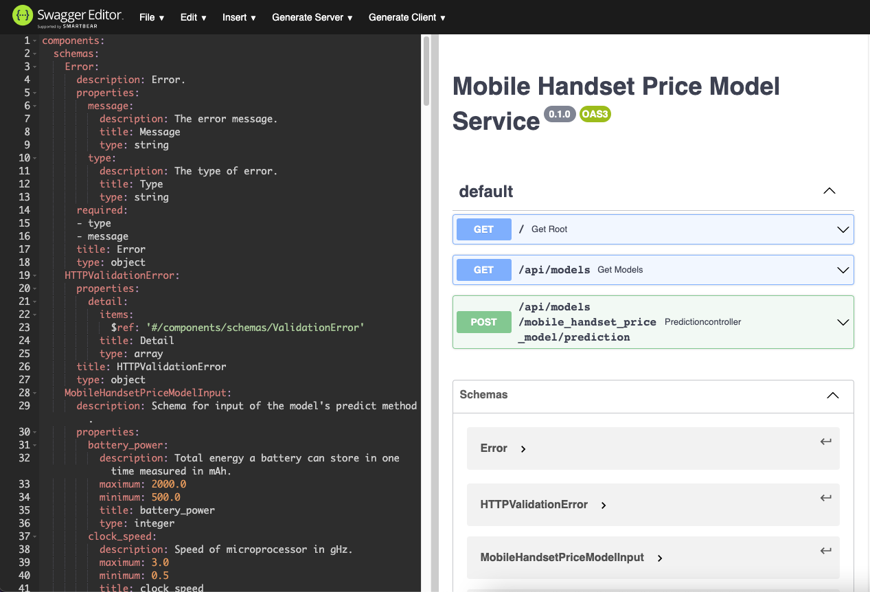
Now that we have the configuration set up, we can automatically generate an OpenAPI specification file for the service, with these commands:
export PYTHONPATH=./
generate_openapi --output_file=service_contract.yaml
The OpenAPI spec file can be found here. We can render the documentation using the Swagger Editor, which looks like this:
The service contract is set up, so now we can run the service locally, with these commands:
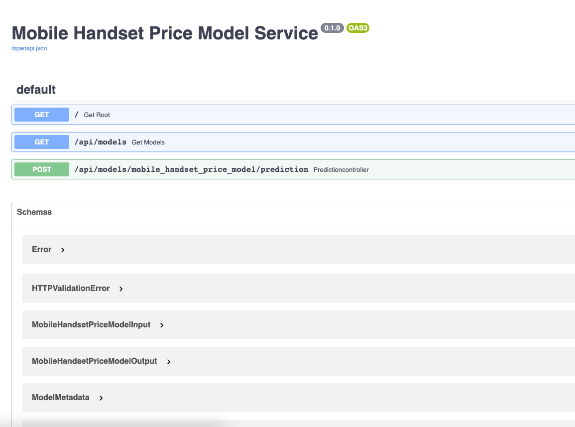
uvicorn rest_model_service.main:app --reload
The service should come up and can be accessed in a web browser at http://127.0.0.1:8000. When you access that URL you will be redirected to the documentation page that is generated by the FastAPI package:
The service is running locally, so now we can try out a request against the model's endpoint:
curl -X 'POST'
'http://127.0.0.1:8000/api/models/mobile_handset_price_model/prediction'
-H 'accept: application/json'
-H 'Content-Type: application/json'
-d '{
"battery_power": 2000,
"has_bluetooth": true,
"clock_speed": 3,
"has_dual_sim": true,
"front_camera_megapixels": 20,
"has_four_g": true,
"internal_memory": 664,
"depth": 1,
"weight": 200,
"number_of_cores": 8,
"primary_camera_megapixels": 20,
"pixel_resolution_height": 1960,
"pixel_resolution_width": 1998,
"ram": 3998,
"screen_height": 19,
"screen_width": 18,
"talk_time": 20,
"has_three_g": true,
"has_touch_screen": true,
"has_wifi": true
}'
The service responds with this result:
{"price_range":"three"}
By using the rest_model_service package we've just set up a RESTful API service that is hosting our model. We can now move on to do property-based testing on the model through the service.
Adding Property-Based API Tests
The schemathesis package allows us to use the hypothesis package against REST API services, doing all of the things that the hypothesis package can do. The schemathesis uses the OpenAPI specification of the service to introspect the service contract and generate test cases.
There are two ways for schemathesis to execute the tests: by sending requests to the service as it runs in its own process or by sending request objects to the ASGI application object as it lives in the memory of a process. The second way is very fast because it does not require that we send requests over the network, so we'll execute the tests that way.
To begin, we'll import the ASGI application object from the rest_model_service package
from rest_model_service.main import app
Next, we'll ask the schemathesis to extract the schema from the application object:
schema = schemathesis.from_asgi("/openapi.json", app, data_generation_methods=[DataGenerationMethod.negative])
Next, we'll generate two strategies from the schema, one strategy per endpoint defined in the application:
model_metadata_strategy = schema["/api/models"]["GET"].as_strategy()

model_prediction_strategy = schema["/api/models/mobile_handset_price_model/prediction"]["POST"].as_strategy()
Now we're ready to start writing the test class:
class APITests(TestCase):

    def setUp(self) -> None:
        self.counter = 0

    def tearDown(self) -> None:
        print("Generated and tested {} examples.".format(self.counter))
The test class keeps track of the number of test cases executed through a counter that is created in the setUp method.
The test case for the metadata endpoint is very simple:
@given(case=model_metadata_strategy)
def test_model_metadata_endpoint(self, case):
    response = case.call_asgi()
    case.validate_response(response)
    self.counter += 1
The \@given decorator uses the model_metadata_strategy to generate test cases for the endpoint. This is a very simple endpoint that does not accept input and provides a static output that contains metadata about the model being hosted in the service.
The next test is much more interesting:
@given(case=model_prediction_strategy)
@settings(max_examples=1000)
def test_model_prediction_endpoint(self, case):
    response = case.call_asgi()
    case.validate_response(response)
    self.counter += 1
The model_prediction_strategy generates test cases for the model's prediction endpoint. The \@settings decorator asks schemathesis to generate 1000 test samples. The case.validate_response() method looks for unexpected responses from the service endpoint.
We executed the api tests with this command:
py.test ./tests/api_tests.py
The command provided this output:
========================== test session starts============================
platform darwin -- Python 3.8.10, pytest-6.2.4, py-1.10.0,
pluggy-0.13.1
rootdir: /Users/brian/Code/property-based-testing-for-ml-models
plugins: pylama-7.7.1, hypothesis-6.14.5, subtests-0.5.0,
schemathesis-3.9.7, anyio-3.3.0, html-3.1.1, metadata-1.11.0
collected 2 items
tests/api_tests.py .. [100%]
======================= 2 passed in 62.51s (0:01:02)===========================
The code for the property-based API tests is in this file.
By executing property-based tests against the model service, we're able to more thoroughly test the model deployment by executing the service code along with the model code in the tests. Although the service code is very simple and lightweight, it helps that we're including it because it makes the hypothesis tests into full integration tests that test the entire service along with the model.
Conclusion
Using property-based tests we were able to find two common errors that can come up when deploying machine learning models. A mismatch between the model's schema and the data that it is actually able to process can cause many issues that are hard to debug. By using this type of generative testing, we were able to find both errors that we introduced to the schema pretty easily.
In this blog post we also saw the benefits of using a package like pydantic for creating the input and output schemas for an ML model. By stating the schemas as code, we're able to clearly show what data is allowed as input and what data is returned by the model. The model's designer does not have to write documentation to explain the input and output data because it is already built into the input and output schema classes.If we didn't have the model's schemas as pydantic classes, the hypothesis and schemathesis packages would not even be able to generate test cases for the model and model service.