Introduction
This post is a collection of several different techniques that I wanted to learn. In this blog post I'll be using open source python packages to do automated data exploration, automated feature engineering, automated machine learning, and model validation. I'll also be using docker and kubernetes to deploy the model. I'll cover the entire codebase of the model, from the initial data exploration to the deployment of the model behind a RESTful API in Kubernetes.
Automated feature engineering is a technique that is used to automate the creation of features from a dataset without having to manually design them and write the code to create the features. Feature engineering is very important for being able to create ML models that work well on a dataset, but it takes a lot of time and effort. Automated feature engineering is able to generate many candidate features from a given dataset, from which we can then select the useful ones. In this blog post, I'll be using the feature_tools library, which helps to do feature preprocessing, feature selection, model selection, and hyperparameter search.
Automated machine learning is a process through which we can create machine learning models without having to explore many different model types and hyperparameters. AutoML can automate the process of choosing the best solution for a dataset, going from a raw dataset to a trained model. AutoML tools allow non-experts to be able to create ML models without having to understand everything that is happening under the hood. All that is needed is a properly processed data set and anyone can generate a model from the data. In this blog post, I'll be using the TPOT library, which helps to do feature preprocessing, feature selection, model selection, and hyperparameter search.
In this blog post, I'll also show how to create a RESTful service for the model that will allow us to deploy the model quickly and simply. We'll also show how to deploy the model service using docker and Kubernetes. This blog post contains a lot of different tools and techniques for building and deploying ML models and it is not meant to be a deep dive into any of the individual techniques, I just wanted to show how to take a model all the way from data exploration, to training and finally to deployment.
Package Structure
The package we'll develop in this blog post has this structure:
- insurance_charges_model
    - model_files (output files from model training)
    - prediction, package for the prediction code
        - __init__.py
        - model.py (prediction code)
        - schemas.py (model input and output schemas)
        - transformers.py (data transformers)
    - training (package for the training code)
        - data_exploration.ipynb (data exploration code)
        - data_preparation.ipynb (data preparation code)
        - model_training.ipynb (model training code)
        - model_validation.ipynb (model validation code)
    - __init__.py
- kubernetes (kubernetes manifests)
    - deployment.yml
    - namespace.yml
    - service.yml
- tests (unit tests for model codel)
- Dockerfile (instructions for generating a docker image)
- Makefile
- requirements.txt (list of dependencies)
- rest_config.yaml (configuration for REST model service)
- service_contract.yaml (OpenAPI service contract)
- setup.py
- test_requirements.txt (test dependencies)
All of the code is available in a github repository.
Getting the Data
In order to train a regression model, we first need to have a dataset. We went into Kaggle and found a dataset that contained insurance charges information. To make it easy to download the data, we installed the kaggle python package. Then we executed these commands to download the data and unzip it into the data folder in the project:
mkdir -p data
kaggle datasets download -d mirichoi0218/insurance -p ./data \--unzip
To make it even easier to download the data, we added a Makefile target for the commands:
download-dataset: ## download dataset from Kaggle
    mkdir -p data
    kaggle datasets download -d mirichoi0218/insurance -p ./data \--unzip
Now all we need to do is execute this command:
make download-data
Instead of having to remember how to get the data needed to do modeling, I always try to create a repeatable and documented process for creating the dataset. We also make sure to never store the dataset in source control, so we'll add this line to the .gitignore file:
data/
Training a Regression Model
Now that we have the dataset, we\'ll start working on training a regression model. We\'ll be doing data exploration, data preparation, feature engineering, automated model training and selection, and model validation.
Exploring the Data
Data exploration is a key step that can tell us a lot about the dataset that we have to model. Data exploration can be highly customized to the specific dataset, but there are also tools that allow us to calculate the most common things we want to learn about a dataset automatically. pandas_profiling is a package that accepts a pandas data frame and creates an HTML report with a profile of the dataset in the data frame. According to the pandas_profiling documentation it has these capabilities:
- Type inference: detect the types of columns in a dataframe.
- Essentials: type, unique values, missing values
- Quantile statistics like minimum value, Q1, median, Q3, maximum, range, interquartile range
- Descriptive statistics like mean, mode, standard deviation, sum, median absolute deviation, coefficient of variation, kurtosis, skewness
- Most frequent values
- Histograms
- Correlations highlighting of highly correlated variables, Spearman, Pearson and Kendall matrices
- Missing values matrix, count, heatmap and dendrogram of missing values
- Duplicate rows Lists the most occurring duplicate rows
- Text analysis learn about categories (Uppercase, Space), scripts (Latin, Cyrillic) and blocks (ASCII) of text data
These are the things that we would be looking into to learn more about the data set. To use the pandas_profiling package, we'll first load the dataset into a pandas dataframe:
import pandas as pd
from pandas_profiling import ProfileReport
data = pd.read_csv("../../data/insurance.csv")
Now we can query the dataframe to find out the column types:
data.dtypes
age int64
sex object
bmi float64
children int64
smoker object
region object
charges float64
dtype: object
To create the profile, we'll execute this code:
profile = ProfileReport(data,
                        title='Insurance Dataset Profile Report',
                        pool_size=4,
                        html={'style': {'full_width': True}})
profile.to_notebook_iframe()
Once the report is created, we'll save it to disk:
profile.to_file("data_exploration_report.html")
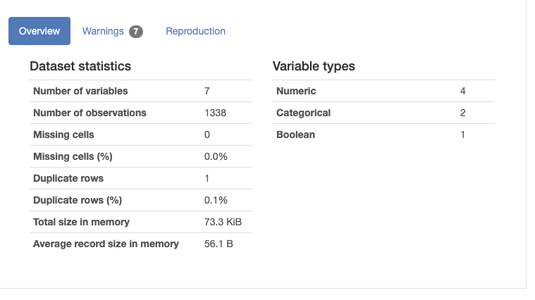
Right away the profile will tell us a few key details about the dataset:
The profile also contains a few warnings about the data:
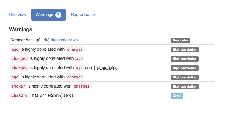
None of these warnings are really that surprising given what we know about insurance charges, since health insurance premiums go up with age, and being a smoker increases your insurance premiums.
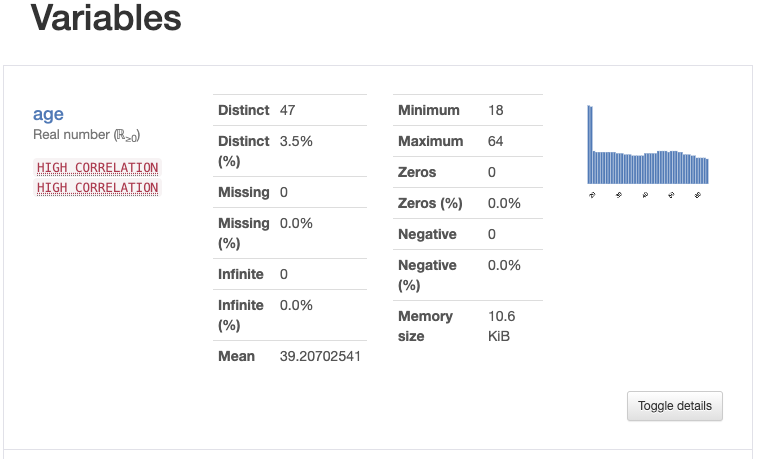
The profile has a description for each variable, here's the description for the age variable:
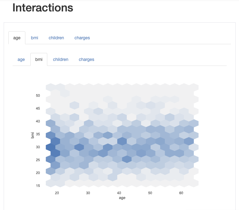
As well as interactions between variables:
And finally the correlations between the variables:
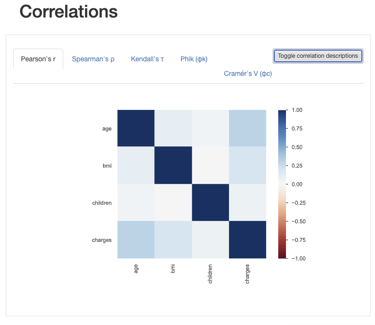
By using the pandas_profiling package we can avoid writing the most common data analysis code that we write for all datasets. All of the code for data exploration is in the data_exploration.ipynb notebook.
Preparing the Data
In order to model the dataset, we'll first need to prepare and preprocess the data. To start, let's load the dataset into a dataframe again:
df = pd.read_csv("../../data/insurance.csv")
To do data preparation, we'll use the feature_tools package to create features from the data that is already in the dataset. To create features, we'll need to tell the feature_tools package about our data by identifying entities in the data:
entityset = ft.EntitySet(id="Transactions")
entityset = entityset.entity_from_dataframe(entity_id="Transactions",
    dataframe=df,
    make_index=True,
    index="index")
In the code above, we created an EntitySet with the id "Transactions" which is the entity that is in the dataframe. The feature_tools package identified the variables associated with the Transactions entity:
entityset["Transactions"].variables
[<Variable: index (dtype = index)>,
<Variable: age (dtype = numeric)>,
<Variable: sex (dtype = categorical)>,
<Variable: bmi (dtype = numeric)>,
<Variable: children (dtype = numeric)>,
<Variable: smoker (dtype = categorical)>,
<Variable: region (dtype = categorical)>,
<Variable: charges (dtype = numeric)>]
We can now generate some new features on the entity:
feature_dataframe, features = ft.dfs(entityset=entityset,
                                     target_entity="Transactions",
                                     trans_primitives=["add_numeric", "subtract_numeric",
                                                       "multiply_numeric", "divide_numeric",
                                                       "greater_than", "less_than"],
                                     ignore_variables={"Transactions": ["sex", "smoker", "region",
                                                                        "charges"]})
The feature_tools package uses a set of primitive operations to generate new features from the data. In this case, we're using the "add_numeric" primitive to generate a new feature by adding up the values in all pairs of numeric variables. By combining numerical variables in this way, we'll generate three new columns:
- age + bmi
- age + children
- bmi + children
The subtract_numeric, multiply_numeric, and divide_numeric primitives also create new columns in a similar way, by applying subtraction, multiplication, and division respectively. The greater_than and less_than primitives create new boolean columns by comparing the values in all pairs of numerical variables. The greater_than primitive generated these new features:
- age > bmi
- age > children
- bmi > age
- bmi > children
- children > age
- children > bmi
At the end of the feature generation, we have 30 new features in the dataset that were generated from the data already there. Before we can use these new features, we need to figure out how to integrate the transformer with scikit-learn pipelines, which is what we will be using to build up our model. To accomplish this we created a transformer which is instantiated like this:
dfs_transformer = DFSTransformer("Transactions",
                                 trans_primitives=["add_numeric", "subtract_numeric",
                                                   "multiply_numeric", "divide_numeric",
                                                   "greater_than", "less_than"],
                                 ignore_variables={"Transactions": ["sex", "smoker",
                                                                    "region"]})
Since the feature generation sometimes creates infinite values, we'll also need a transformer to convert these to nan values. This transformer is instantiated like this:
infinity_transformer = InfinityToNaNTransformer()
To handle the nan values generated by the InfinityToNaN transformer, we'll use a SimpleImputer from the scikit-learn library. It is instantiated like this:
simple_imputer = SimpleImputer(missing_values=np.nan, strategy='mean')
The SimpleImputer transformer has problems with imputing values that are not floats when using the \'mean\' strategy. To fix this, we\'ll create a transformer that will convert all integer columns into floating point columns:
int_to_float_transformer = IntToFloatTransformer()
Lastly, we\'ll put the DFSTransformer, IntToFloatTransformer, InfinityToNaNTransformer, and SimpleImputer transformers into a Pipeline so they\'ll all work together as a unit:
dfs_pipeline = Pipeline([
    ("dfs_transformer", dfs_transformer),
    ("int_to_float_transformer", int_to_float_transformer),
    ("infinity_transformer", infinity_transformer),
    ("simple_imputer", simple_imputer),
])
Next, we'll deal with the boolean features in the dataset. To do this, we created a transformer that converts string values into the corresponding true or false values. It's instantiated like this:
boolean_transformer = BooleanTransformer(true_value="yes", false_value="no")
This transformer will be used to convert the "smoker" variable into a boolean value. The values found in the dataset are "yes" and "no". The encoder is configured to convert "yes" to True, and "no" to False.
Next, we\'ll create an encoder that will encode the categorical features. The categorical features that we will encode will be \'sex\' and \'region\'. We'll use the OrdinalEncoder from the scikit-learn library:
ordinal_encoder = OrdinalEncoder()
Now we can create a ColumnTransformer that combines all of the pipelines and transformers we created above into one bigger pipeline:
column_transformer = ColumnTransformer(remainder="passthrough",
                                       transformers=[
                                           ("dfs_pipeline", dfs_pipeline, ["age", "sex", "bmi",
                                                                           "children", "smoker", "region"]),
                                           ("boolean_transformer", boolean_transformer, ["smoker"]),
                                           ("ordinal_encoder", ordinal_encoder, ["sex", "region"])
                                       ])
The ColumnTransformer applies the deep feature synthesis pipeline to all of the input variables, then it applies the boolean transformer to the "smoker" variable, and the ordinal encoder to the "sex" and "region" variables.
Now we do a small test to make sure that the transformations are happening as expected:
test_df = pd.DataFrame([[65, "male", 12.5, 0, "yes", "southwest"],
                        [75, "female", 78.770, 1, "no", "southeast"]],
                       columns=["age", "sex", "bmi", "children", "smoker", "region"])

column_transformer.fit(test_df)

result = column_transformer.transform(test_df)

if len(result[0]) != 33: # expecting 33 features to come out of the ColumnTransformer
    raise ValueError("Unexpected number of columns found in the dataframe.")
To test the pipeline, we created a dataframe with two rows, then we fitted the pipeline to it and transformed the dataframe. We expect to get 33 columns in the output dataframe because of the deep feature synthesis, so we test for that and raise an exception if it is not the case.
The columns transformer can now be saved so we can use it later in the model training process:
joblib.dump(column_transformer, "transformer.joblib")
In this section we used scikit-learn pipelines to compose a complex series of data transformations that will be executed when the model is trained and also when it is used for predictions. By using pipelines, we are able to make sure that the steps always happen in the same order and with the same parameters. If we didn't use pipelines, we would end up rewriting the transformations twice, once for model training and once for prediction. All of the code for data preparation is in the data_preparation.ipynb notebook.
Training a Model
The next step after preparing the data is to train a model. For this, we'll use the TPOT package, which is an automated machine learning tool that is able to search through many possible model types and hyperparameters and find the best pipeline for the dataset. The package uses genetic programming to search the space of possible ML pipelines.
To train the model, we'll first load the dataset:
df = pd.read_csv("../../data/insurance.csv")
Then, we'll create a training set and a test set by randomly selecting samples. The training testing split will be 80:20.
mask = np.random.rand(len(df)) < 0.8
training_set = df[mask]
testing_set = df[~mask]
Next, we'll save the data sets to the data folder because we'll need the two datasets when we do model validation. Since we're choosing to do this in another Jupyter notebook, we need to keep the data sets on the hard drive until then.
training_set.to_csv("../../data/training_set.csv")
testing_set.to_csv("../../data/testing_set.csv")
Now that we have a training set, we'll need to separate the feature columns from the target column:
feature_columns = ["age", "sex", "bmi", "children", "smoker", "region"]
target_column = "charges"
X_train = training_set[feature_columns]
y_train = training_set[target_column]
X_test = testing_set[feature_columns]
y_test = testing_set[target_column]
Next, we'll apply the preprocessing pipeline that we built in the data preprocessing code. First we'll load the transformer that we saved to disk:
transformer = joblib.load("transformer.joblib")
Now we can apply it to the features dataframe in order to calculate the features that we created using automated feature engineering:
features = transformer.fit_transform(X_train)
Now that we have a features dataframe that we can train a model with, we'll launch the training by instantiating a TPOTRegressor object and calling the fit method:
tpot_regressor = TPOTRegressor(generations=50,
                               population_size=50,
                               random_state=42,
                               cv=5,
                               n_jobs=8,
                               verbosity=2,
                               early_stop=10)

tpot_regressor = tpot_regressor.fit(features, y_train)
The TPOTRegressor uses genetic programming so we need to provide some parameters that will define the size of the population and the number of generations. The random_state parameter makes it easier to replicate the training run, the cv parameter is the number of cross validation splits that we want to use, the n_jobs parameters tells TPOT how many processes to launch to train the model.
Here is a sample of the output of the tpot_regressor as it trains:
Optimization Progress: 100%
2550/2550 [35:22<00:00, 1.15pipeline/s]
Generation 1 - Current best internal CV score: -19328040.90181576
Generation 2 - Current best internal CV score: -19328040.90181576
Generation 3 - Current best internal CV score: -19291161.694311526
Generation 4 - Current best internal CV score: -19216662.844604537
Generation 5 - Current best internal CV score: -19194856.36477192

...

Generation 48 - Current best internal CV score: -18848299.473418456
Generation 49 - Current best internal CV score: -18848299.473418456
Generation 50 - Current best internal CV score: -18848299.473418456

Best pipeline:
RandomForestRegressor(MaxAbsScaler(SGDRegressor(Normalizer(input_matrix,
norm=l2), alpha=0.01, eta0=1.0, fit_intercept=True, l1_ratio=0.0,
learning_rate=invscaling, loss=squared_loss, penalty=elasticnet,
power_t=0.1)), bootstrap=True, max_features=0.7500000000000001,
min_samples_leaf=16, min_samples_split=14, n_estimators=100)
It looks like the best pipeline found by TPOT includes a RandomForestRegressor combined with several preprocessing steps. Now that we have an optimal pipeline created by TPOT we will be adding our own preprocessors to it. To do this we\'ll need to have an unfitted pipeline object, we don\'t have that right now because the TPOTRegressor pipeline has been fitted.
To get an unfitted pipeline we\'ll ask TPOT for the fitted pipeline and clone it:
unfitted_tpot_regressor = clone(tpot_regressor.fitted_pipeline_)
Now that we have an unfitted Pipeline that is the same pipeline that was found by the TPOT package, we\'ll add our own preprocessors to the pipeline. This will ensure that the final pipeline will accept the features in the original dataset and will process the features correctly. We\'ll compose the unfitted TPOT pipeline and the transformer Pipeline into one Pipeline:
model = Pipeline([("transformer", transformer),
                  ("tpot_pipeline", unfitted_tpot_regressor)
                  ])
Now we can train the model on the original, unprocessed dataset:
model.fit(X_train, y_train)
The final fitted pipeline contains all of the transformations that we used to do deep feature synthesis and data preprocessing, and all of the transformations that were added by TPOT. This is the final pipeline:
Pipeline(steps=[('transformer',
                 ColumnTransformer(remainder='passthrough',
                                   transformers=[('dfs_pipeline',
                                                  Pipeline(steps=[('dfs_transformer',
                                                                   DFSTransformer(ignore_variables={'Transactions': ['sex',
                                                                                                                     'smoker',
                                                                                                                     'region']},
                                                                                  target_entity='Transactions',
                                                                                  trans_primitives=['add_numeric',
                                                                                                    'subtract_numeric',
                                                                                                    'multiply_numeric',
                                                                                                    'divide_numeric',
                                                                                                    'greater_than',
                                                                                                    'less_...
                                                                                                    Pipeline(steps=[('normalizer', Normalizer()),
                                                                                                                    ('stackingestimator',
                                                                                                                     StackingEstimator(estimator=SGDRegressor(alpha=0.01,
                                                                                                                                                              eta0=1.0,
                                                                                                                                                              l1_ratio=0.0,
                                                                                                                                                              penalty='elasticnet',
                                                                                                                                                              power_t=0.1,
                                                                                                                                                              random_state=42))),
                                                                                                                    ('maxabsscaler', MaxAbsScaler()),
                                                                                                                    ('randomforestregressor',
                                                                                                                     RandomForestRegressor(max_features=0.7500000000000001,
                                                                                                                                           min_samples_leaf=16,
                                                                                                                                           min_samples_split=14,
                                                                                                                                           random_state=42))]))])
Finally, we'll test the model with a single sample:
test_df = pd.DataFrame([[65, "male", 12.5, 0, "yes", "southwest"]],
columns=["age", "sex", "bmi", "children", "smoker", "region"])
result = model.predict(test_df)
The result is:
array([19326.59077456])
In order to use the model later, we'll serialize it to disk:
joblib.dump(model, "model.joblib")
All of the code for training the model is in the model_training.ipynb notebook.
Validating the Model
In order to validate the model generated by the autoML process, we'll use the yellow_brick library.
First, we'll load the training and testing sets that we previously saved to disk:
training_set = pd.read_csv("../../data/training_set.csv")
testing_set = pd.read_csv("../../data/testing_set.csv")
Next, we'll separate the predictor variables from the target variable:
feature_columns = ["age", "sex", "bmi", "children", "smoker", "region"]
target_column = "charges"
X_train = training_set[feature_columns]
y_train = training_set[target_column]
X_test = testing_set[feature_columns]
y_test = testing_set[target_column]
We'll load the fitted model object that was saved in a previous step:
model = joblib.load("model.joblib")
We can now try to make predictions on the test set with the fitted pipeline:
predictions = model.predict(X_test)
The model's r\^2 and errors are calculated like this:
r2 = r2_score(y_test, predictions)
mse = mean_squared_error(y_test, predictions)
mae = mean_absolute_error(y_test, predictions)
The results are:
r2 score: 0.827414647586443
mean squared error: 24830561.579995826
mean absolute error: 2713.6533067216383
Next, we'll create a yellow_brick visualizer for the model:
visualizer = ResidualsPlot(model)
visualizer.fit(X_train, y_train)
visualizer.score(X_test, y_test)
visualizer.show()
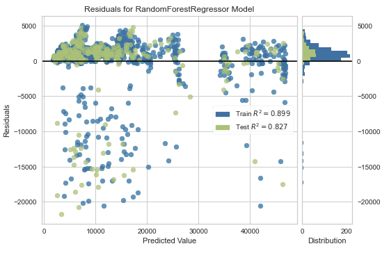
The ResidualsPlot visualizer shows us the difference between the observed value and the predicted value of the target variable. This visualization is useful to see if there are value ranges for the target variable that have more or less error than other value ranges. The plot generated for our model looks like this:
Next, we'll generate the prediction error plot for the model using the PredictionError visualizer:
visualizer = PredictionError(model)
visualizer.fit(X_train, y_train)
visualizer.score(X_test, y_test)
visualizer.show()
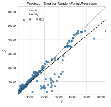
The prediction error plot shows the actual values of the target variable against the predicted values generated by the model. This allows us to see how much variance is in the predictions made by the model. The plot generated for our model looks like this:
All of the code for validating the model is in the model_validation.ipynb notebook.
Making Predictions with the Model
The insurance charges model is now ready to be used to make predictions, so now we need to make it available in an easy to use format. The ml_base package defines a simple base class for model prediction code that allows us to "wrap" the code in a class that follows the MLModel interface. This interface publishes this information about the model:
- Qualified Name, a unique identifier for the model
- Display Name, a friendly name for the model used in user interfaces
- Description, a description for the model
- Version, semantic version of the model codebase
- Input Schema, an object that describes the model\'s input data
- Output Schema, an object that describes the model\'s output schema
The MLModel interface also dictates that the model class implements two methods:
- __init__, initialization method which loads any model artifacts needed to make predictions
- predict, prediction method that receives model inputs makes a prediction and returns model outputs
By using the MLModel base class we'll be able to do more interesting things later with the model. If you'd like to learn more about the ml_base package, there is a blog post about it.
To install the ml_base package, execute this command:
pip install ml_base
Creating Input and Output Schemas
Before writing the model class, we'll need to define the input and output schemas of the model. To do this, we'll use the pydantic package.
The "sex" feature used by the model is a categorical feature that can be stated as an enumeration because it has a limited number of allowed values:
class SexEnum(str, Enum):
    male = "male"
    female = "female"
We'll use this class as a type in the input schema of the model.
We'll also need another enumeration for the region feature:
class RegionEnum(str, Enum):
    southwest = "southwest"
    southeast = "southeast"
    northwest = "northwest"
    northeast = "northeast"
Now we're ready to create the input schema for the model:
class InsuranceChargesModelInput(BaseModel):
    age: int = Field(None, title="Age", ge=18, le=65, description="Age of primary beneficiary in years.")
    sex: SexEnum = Field(None, title="Sex", description="Gender of beneficiary.")
    bmi: float = Field(None, title="Body Mass Index", ge=15.0, le=50.0, description="Body mass index of beneficiary.")
    children: int = Field(None, title="Children", ge=0, le=5, description="Number of children covered by health insurance.")
    smoker: bool = Field(None, title="Smoker", description="Whether beneficiary is a smoker.")
    region: RegionEnum = Field(None, title="Region", description="Region where beneficiary lives.")
We used the SexEnum and RegionEnum as types for the categorical variables, adding descriptions to the fields. We also added the age, bmi, children, and smoker fields. These fields are of type integer, float, integer, and boolean in turn.
We can use the class to create an object like this:
from insurance_charges_model.prediction.schemas import InsuranceChargesModelInput

input = InsuranceChargesModelInput(age=22, sex="male", bmi=20.0, children=0, region="southwest")
Now that we have the model input defined, we'll move on to the model output. This class is a lot simpler:
class InsuranceChargesModelOutput(BaseModel):
    charges: float = Field(None, title="Charges", description="Individual medical costs billed by health insurance to customer in US dollars.")
The model only has one output, the charges in US dollars that are predicted, which is a floating point field. The model schemas are in the schemas module in the prediction package.
Creating the Model Class
Since we now have the input and output schemas defined for the model, we'll be able to create the class that wraps around the model.
To start, we'll define the class and add all of the required properties:
class InsuranceChargesModel(MLModel):
    @property
    def display_name(self) -> str:
        return "Insurance Charges Model"

    @property
    def qualified_name(self) -> str:
        return "insurance_charges_model"

    @property
    def description(self) -> str:
        return "Model to predict the insurance charges of a customer."

    @property
    def version(self) -> str:
        return __version__

    @property
    def input_schema(self):
        return InsuranceChargesModelInput

    @property
    def output_schema(self):
        return InsuranceChargesModelOutput
The properties are required by the MLModel base class and they are used to easily access metadata about the model. The input and output schema classes are returned from the input_schema and output_schema properties.
The __init__ method of the class looks like this:
def __init__(self):
    dir_path = os.path.dirname(os.path.dirname(os.path.realpath(__file__)))

    with open(os.path.join(dir_path, "model_files", "1", "model.joblib"), 'rb') as file:
        self._svm_model = joblib.load(file)
The init method is used to load the model parameters from disk and store the model object as an object attribute. The model object will be used to make predictions. Once the init method completes, the model object should be initialized and ready to make predictions.
The prediction method of the model class looks like this:
def predict(self, data: InsuranceChargesModelInput) -> InsuranceChargesModelOutput:
    X = pd.DataFrame([[data.age, data.sex.value, data.bmi, data.children, data.smoker, data.region.value]],
                     columns=["age", "sex", "bmi", "children", "smoker", "region"])

    y_hat = round(float(self._svm_model.predict(X)[0]), 2)

    return InsuranceChargesModelOutput(charges=y_hat)
The predict method accepts an object of type InsuranceChargesModelInput and returns an object of type InsuranceChargesModelOutput. First, the method converts the incoming data into a pandas dataframe, then the dataframe is used to make a prediction, and the result is converted to a floating point number and rounded to two decimal places. Lastly, the output object is created using the prediction and returned to the caller.
The model class is defined in the model module in the prediction package.
Creating a RESTful Service
Now that we have a model class defined, we are finally able to build the RESTful service that will host the model when it is deployed. Luckily, we don't actually need to write any code for this because we'll be using the rest_model_service package. If you'd like to learn more about the rest_model_service package, there is a blog post about it.
To install the package, execute this command:
pip install rest_model_service
To create a service for our model, all that is needed is that we add a YAML configuration file to the project. The configuration file looks like this:
service_title: Insurance Charges Model Service
models:
  - qualified_name: insurance_charges_model
    class_path: insurance_charges_model.prediction.model.InsuranceChargesModel
    create_endpoint: true
The service title is the name we'll give the service in the documentation. The models array contains references to the models that we'd like to host within the service. Each model needs to have the qualified name of the model along with the class path to the model's MLModel class. The create_endpoint option is set to true to tell the service to create an endpoint for the model.
Using the configuration file, we're able to create an OpenAPI specification file for the model service by executing this command:
export PYTHONPATH=./
generate_openapi \--output_file=service_contract.yaml
The service_contract.yaml file will be generated and it will contain the specification that was generated for the model service. The insurance_charges_model endpoint is the one we'll call to make predictions with the model. The model's input and output schemas were automatically extracted and added to the specification.
To run the service locally, execute these commands:
uvicorn rest_model_service.main:app \--reload
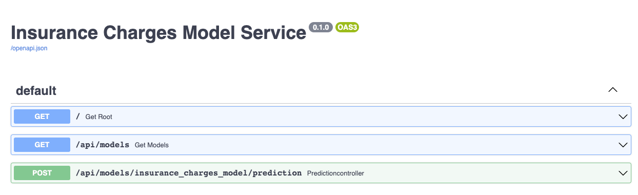
The service should come up and can be accessed in a web browser at http://127.0.0.1:8000. When you access that URL you will be redirected to the documentation page that is generated by the FastAPI package:
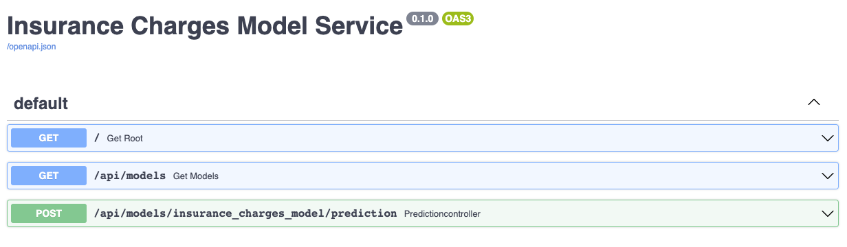
The documentation allows you to make requests against the API in order to try it out. Here's a prediction request against the insurance charges model:
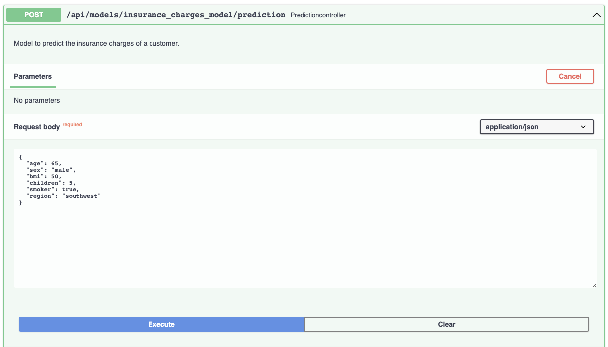
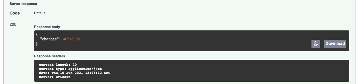
And the prediction result:
By using the MLModel base class provided by the ml_base package and the REST service framework provided by the rest_model_service package we're able to quickly stand up a service to host the model.
Deploying the Model
Now that we have a working model and model service, we'll need to deploy it somewhere. To do this, we'll use docker and kubernetes.
Creating a Docker Image
Before moving forward, let's create a docker image and run it locally. The docker image is generated using instructions in the Dockerfile:
FROM tiangolo/uvicorn-gunicorn-fastapi:python3.7

MAINTAINER Brian Schmidt
"6666331+schmidtbri@users.noreply.github.com"

WORKDIR ./service

COPY ./insurance_charges_model ./insurance_charges_model
COPY ./rest_config.yaml ./rest_config.yaml
COPY ./service_requirements.txt ./service_requirements.txt

RUN pip install -r service_requirements.txt

ENV APP_MODULE=rest_model_service.main:app
The Dockerfile is used by this command to create the docker image:
docker build -t insurance_charges_model:0.1.0 .
To make sure everything worked as expected, we'll look through the docker images in our system:
docker image ls
The insurance_charges_model image should be listed. Next, we'll start the image to see if everything is working as expected:
docker run -d -p 80:80 insurance_charges_model:0.1.0
The service should be accessible on port 80 of localhost, so we'll try to make a prediction using the curl command:
curl -X 'POST' \
'http://localhost/api/models/insurance_charges_model/prediction' \
-H 'accept: application/json' \
-H 'Content-Type: application/json' \
-d '{
"age": 65,
"sex": "male",
"bmi": 50,
"children": 5,
"smoker": true,
"region": "southwest"
}'
We got back this output, which tells us that the service is working as expected:
{"charges":46918.68}
If there are any problems, we should be able to debug them using the logs. To see the logs emitted by the running container, execute this command:
docker logs $(docker ps -lq)
To stop the docker container, execute this command:
docker kill $(docker ps -lq)
Setting up Digital Ocean
To show how to deploy the model service we created, we'll use Digital Ocean. In this section we'll be using the doctl command line utility which will help us to interact with the Digital Ocean Kubernetes service. We followed these instructions to install the doctl utility. Before we can do anything with the Digital Ocean API, we need to authenticate, so we created an API token by following these instructions. Once we have the token we can add it to the doctl utility by creating a new authentication context with this command:
doctl auth init \--context model-services-context
The command creates a new context called "model-services-context" that we'll use to interact with the Digital Ocean API. The command asks for the API token we generated and saves it into the configuration file of the tool. To make sure that the context was created correctly and is the current context, execute this command:
doctl auth list
If the context we created is not the current context, we can switch to it with this command:
doctl auth switch \--context model-services-context
To make sure that we are working in the right account, execute this command:
doctl account get
The account details should match the account that you used to login. Now that we are connecting to the right account in DO, we'll work on uploading the docker image that contains the model service so that we can use it in the Kubernetes cluster. First, we'll create a container registry with this command:
doctl registry create model-services-registry \--subscription-tier basic
We called the new registry "model-services-registry" and we used the basic tier, which costs \$5 a month.
Pushing the Image
Now that we have a registry, we need to add credentials to our local docker daemon in order to be able to upload images, to do that we'll use this command:
doctl registry login
In order to upload the image, we need to tag it with the URL of the DO registry we created. The docker tag command looks like this:
docker tag insurance_charges_model:0.1.0
registry.digitalocean.com/model-services-registry/insurance_charges_model:0.1.0
Now we can push the image to the DO registry:
docker push registry.digitalocean.com/model-services-registry/insurance_charges_model:0.1.0
Creating the Kubernetes Cluster
The doctl tool provides an option for creating a Kubernetes cluster, the command goes like this:
doctl kubernetes cluster create model-services-cluster
The cluster should come up after a while. The default cluster size is 3 nodes which should cost about \$30 to run for a month. We'll shut the cluster down later to save money.
Next, we need to add Kubernetes integration with Digital Ocean's docker registry, this allows the kubernetes cluster to pull images from the docker registry we created above. To do this execute this command:
doctl kubernetes cluster registry add model-services-cluster
To access the cluster, doctl has another option that will set up the kubectl tool for us:
doctl kubernetes cluster kubeconfig save 85866655-708d-47a9-8797-bcca56a10401
The unique identifier is for the cluster that was just created and is returned by the previous command. When the command finishes, the current context in kubectl should be switched to the newly created cluster. To list the contexts in kubectl, execute this command:
kubectl config get-contexts
A listing of the contexts currently in the kubectl configuration should appear, and there should be a star next to the new cluster's context. We can get a list of the nodes in the cluster with this command:
kubectl get nodes
Now that we have a cluster and are connected to it, we'll create a namespace to hold the resources for our model deployment. We'll create a namespace using this YAML manifest:
apiVersion: v1
  kind: Namespace
  metadata:
  name: model-services-namespace
The manifest can be found in this file. To apply the manifest to the cluster, execute this command:
kubectl create -f kubernetes/namespace.yml
To take a look at the namespaces, execute this command:
kubectl get namespace
The new namespace should appear in the listing along with other namespaces created by default by the system. To use the new namespace for the rest of the operations, execute this command:
kubectl config set-context --current --namespace=model-services-namespace
Creating a Kubernetes Deployment
We are now ready to actually create a deployment in the cluster. A deployment is a resource created within the Kubernetes cluster that provides declarative updates to individual pods and ReplicaSets. A pod represents a single instance of the web service that is hosting our model. We'll use a Deployment to launch two instances of the service in the cluster. The Deployment will manage the state of the Pods that hold the service instances and make sure that the desired state is always maintained in the cluster.
The Deployment is defined as YAML like this:
apiVersion: apps/v1
kind: Deployment
metadata:
  name: insurance-charges-model-deployment
  labels:
    app: insurance-charges-model
spec:
  replicas: 1
  selector:
    matchLabels:
      app: insurance-charges-model
  template:
    metadata:
      labels:
        app: insurance-charges-model
    spec:
      containers:
        - name: insurance-charges-model
          image: registry.digitalocean.com/model-services-registry/insurance_charges_model:0.1.0
          ports:
          - containerPort: 80
            protocol: TCP
          imagePullPolicy: Always
          resources:
            requests:
              cpu: "250m"
The file containing the YAML is here. The deployment specifies that there should be two replicas of the docker image running in the cluster. The "app=insurance-charges-model" is applied to the two Pods and is used to select them later.
The Deployment is created within the Kubernetes cluster with this command:
kubectl apply -f kubernetes/deployment.yml
Once the command finishes we can see the new deployment with this command:
kubectl get deployments
We can view the pods that are being managed by the deployment with this command:
kubectl get pods
The output should look something like this:
NAME    READY   STATUS  RESTARTS    AGE
insurance-charges-model-deployment-7d58f6d569-zwjpw 1/1 Running 0 3m48s
Creating a Kubernetes Service
Now that we have a set of pods, we need to make them accessible to the outside world. The Service resource within Kubernetes is used to select a set of Pods and allow access to them through a single entry point. The Service allows us to decouple the Pods and Deployment resources that make up our REST service from the way that they are exposed to users.
The Service is defined as YAML like this:
apiVersion: v1
kind: Service
metadata:
  name: insurance-charges-model-service
spec:
  type: LoadBalancer
  selector:
    app: insurance-charges-model
  ports:
    - name: http
      protocol: TCP
      port: 80
      targetPort: 80
The YAML file is here. The Service is selecting the same Pods that are managed by the Deployment resource which we created above by using the same selector.
The Service is created within the Kubernetes cluster with this command:
kubectl apply -f kubernetes/service.yml
You can see the new service with this command:
kubectl get services
The Service type is LoadBalancer, which means that the cloud provider is providing a load balancer and public IP address through which we can contact the service. To view details about the load balancer provided by Digital Ocean for this Service, we'll execute this command:
kubectl describe service insurance-charges-model-service | grep "LoadBalancer Ingress"
The load balancer can take a while longer than the service to come up, until the load balancer is running the command won't return anything. The IP address that the Digital Ocean load balancer sits behind will be listed in the output of the command. To get access to the service, we'll hit the IP address with a web browser:
We can access the service documentation through the load balancer and the Pod that is running the REST service is returning the webpage.
We'll try the same curl command as before to see if the model is reachable:
curl -X 'POST' 'http://143.244.214.226/api/models/insurance_charges_model/prediction' \
-H 'accept: application/json' \
-H 'Content-Type: application/json' \
-d '{
"age": 65,
"sex": "male",
"bmi": 50,
"children": 5,
"smoker": true,
"region": "southwest"
}'
A prediction was returned from the model:
{"charges":46277.67}
Deleting the Resources
Now that we're done with the service we need to destroy the resources. To destroy the load balancer, execute this command:
doctl compute load-balancer delete \--force $(kubectl get svc insurance-charges-model-service -o jsonpath="{.metadata.annotations.kubernetes\.digitalocean\.com/load-balancer-id}")
To destroy the kubernetes cluster, execute this command:
doctl k8s cluster delete 85866655-708d-47a9-8797-bcca56a10401
To destroy the docker registry, execute this command:
doctl registry delete model-services-registry
Closing
This blog post was created as a demonstration of how to build and deploy machine learning models quickly and easily. Although I didn\'t do any deep explanations of how the different tools work, I made sure to link to other resources from which you can learn more about them. The techniques and packages used are all open source and can be easily downloaded and used in other projects.
The dataset that we used happens to be useful for predicting insurance charges, but the code in this project can be used to train a model based on any regression data set because of the automated feature engineering and automated machine learning techniques that we used. We should be able to throw any dataset at the code and the automations that we built will enable us to quickly build a model and deploy a RESTful service with it.
Something that we can improve on in the future is to create a Helm chart that we can use to deploy an ML model service quickly and easily. Since the Kubernetes resources for the model service are likely to be very similar to other model services, we should be able to create a Helm chart that we can reuse to quickly spin up model services that follow the same pattern as this one.
Another thing that we can improve on is the automated generation of input and output schemas for the model. When we built the input and output schemas for the model, we had to manually extract the field information from the dataframes. By introspecting the dataframe metadata, we should be able to automatically generate the input and output schemas, which can be used to automatically generate the code in the schemas.py module. This is just one way in which we can further automate the deployment process of an ML model.